(2009) pp. 103–110
http://ami.ektf.hu
Localization of touching points for interpolation of discrete circles
Roland Kunkli
Department of Computer Graphics and Image Processing University of Debrecen, Hungary
Submitted 17 February 2009; Accepted 8 May 2009
Abstract
Interpolation of an ordered set of discrete circles is discussed in this paper.
By interpolation here we mean the construction of two curves which touch each of the circles and provide visually satisfactory result. Existing method frequently fail, and the crucial problem is to find good touching points on the circles. In this paper we will consider two possible solutions with pros and drawbacks.
Keywords: interpolation, circles, cyclography MSC:68U05
1. Introduction
Interpolation of geometric data sets is of central importance in Computer Aided Geometric Design. If geometric data consist of points, then we have standard meth- ods to interpolate them [2, 3, 4] which give a uniquely defined fix curve. There are also recently developed methods where one can alter the shape of the interpolating curve [5, 6, 7, 8]. If, however, data set consists of other types of objects, interpo- lation is transferred to skinning or enveloping, and there is no unified method to solve the problem.
In this paper we address the problem of interpolation of a sequence of circles at arbitrarily given positions and radii. By interpolation we mean the construction of a pair of curves which touch the circles and the result is visually satisfactory, i.e.
there are no unnecessary oscillations, bumps and loops on the curves.
This or similar problem - beside its theoretical interest - frequently arises in ap- plications like designing tubular structures, covering problems, molecule modeling, sometimes in 3D [11], [12].
103
Figure 1: Position of circles where theoretically impossible to find skinning envelopes (circle No. 2 and 4)
Figure 2: Position of circles where the existence of skinning enve- lope is theoretically possible
The sequence of circles has to satisfy a natural condition: we exclude circles which are entirely inside of other circles (c.f. Fig. 1). In Fig. 2, however we can see that small changes yield permissible positions. Otherwise the positions and radii of circles can arbitrarily be chosen.
From this point we exclude the numbering of circles from Figures - sequence starts from left to right.
Two recent approaches of the problem can be found in [9] and [10]. The first one is based on the theoretical results of envelope design of various families of curves, but as we will show in the next section, the method basically works only if one or two-parameter family of curves are given, for discrete sequences of curves the method may provide unsatisfactory result. For discrete case Slabaugh et al.
provided a numerical, iterative method in [10], which works well if the radii and positions of curves do not change suddenly, that is the given data are fairly smooth.
In Section 2 we will also show positions of curves for which the method simply fails, providing unnecessary oscillations and singularities.
In interpolation of circles the crucial problem is to find the touching points. In Section 3 we describe two alternative methods, each of which works well in most of the cases, even if the above mentioned methods do not work, but may fail in some extreme circumstances. Conclusions and possible further improvements close the paper.
2. Related works
Slabaugh’s method is an iterative way to construct the desired curves. Let the discrete sequence of curves with centersciand radiiri,(i= 1, . . . , n)be given. Ini- tially pairs of Hermite arcs are defined between the consecutive circles. Considering e.g. theithand(i+ 1)thcircles, two Hermite arcs are defined with touching points pi,pi+1 and tangents ti,ti+1 for the two arcs, separately. The final positions of these points and tangents are obtained by the end of the iteration steps.
Figure 3: A good result by Slabaugh’s method (from [10])
The iteration itself based on the minimization of a predefined energy function.
For computational reasons the positions of the touching points and the tangents are transferred into one single variable, namely the angle αi between the x axis and the radius pointing towards the touching point.
pi=ci+
ricosαi
risinαi
,
ti=
−kisinαi
kicosαi
,
where ki is a predefined constant for each circle, half of the distance between the centers ci andci+1.
Figure 4: Automatic initial values of Slabaugh’s method can yield unacceptable result even for simple data set (from [10]).
The method gives acceptable result if the sequence of curves form a "smooth"
data set (c.f. Fig. 3), but even this case the initialization of the iteration, that is
the starting values of the angles αi requires user interaction, otherwise automatic values can yield obviously wrong result as one can observe in Fig. 4. A further problem is that the convergence is not proved, the number of iteration can be over 100.
Figure 5: Peternell’s method applies cyclographic mapping and spatial interpolation. Perspective and upper view of data circles
and interpolation curve
Peternell’s method is based on a cyclographic approach. Cyclography defines a one-to-one correspondence between the oriented circles of the plane and the spatial points by cones. This way the sequence of given circles can be transformed to a sequence of spatial points (c.f. Fig. 5). An interpolating curve through these points can be defined by any standard method and finally points of this spatial curve can be transferred back to circles on the plane by he cones. The envelope of these circles is obtained as the intersection of the plane and the envelope surface of the cones. For a more detailed description, see [9], [13].
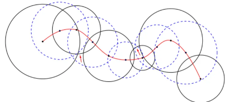
Figure 6: Classical interpolation may yields circles where the enve- lope cannot be constructed (positions pointed by red arrows), that
is Peternell’s method cannot be applied
Although this method solves the problem theoretically, it works perfectly only in the case if we know a one- or two-parameter set of circles, i.e. instead of the discrete circles(ci, ri),i= 1, . . . , n, two functionsc(t), r(t)are given.
Although these functions can be achieved from the set of discrete circles by classical interpolating methods, but this way the method not necessarily gives ap-
propriate result, as one can observe in Fig. 6. The interpolation curve is computed byC1 continuous Hermite arcs.
3. New methods for determining touching points
As we have learned from the previous section, the localization of possible touch- ing points on the given circles is essential for good interpolation. In this section we discuss two methods to find these points. Although these techniques are not perfect, the second one gives acceptable results even for some extreme positions of data, for which the above mentioned methods may fail.
3.1. Planar curve driven method
The first and maybe the most natural approach is to start from a curve which interpolates the centers ci,(i= 1, . . . , n)of the given curves. For these points C1 continuous Hermite arcs is constructed, using Bessel’s method to construct the tangent vectorsvi at the centers ci.
Figure 7: The planar curve driven method provides suitable touch- ing in most cases
Now at each center consider a line orthogonal to the tangent line and consider the intersection points of this line and the corresponding circle. This method gives two pointsp1,i,p2,iat each circle:
p1,i=ci+vi(90◦)
|vi| ri, p2,i=ci+vi(−90◦)
|vi| ri,
where vi(α) denotes the vector obtained by rotating the vector vi with angle α. Thus to distinguish the points on one circle, we use the orientation derived from the Hermite arcs.
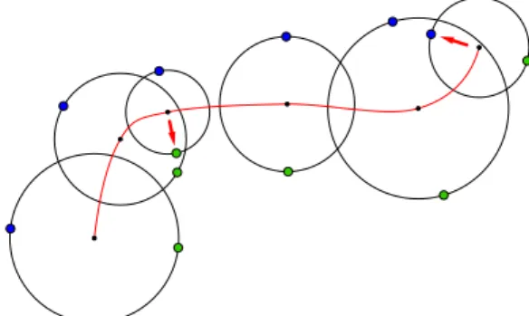
Figure 8: Sometimes computed touching points can fall into other circles
This way the two sequences of points p1,i and p2,i may serve us as touching points of the future interpolation curves. This method gives satisfactory result in several cases (Fig. 7), but sometimes the points p1,i orp2,i can fall into other circles (Fig. 8).
3.2. Spatial curve driven method
As we have seen in Section 2, circles can be transformed to spatial points by the cyclographical method. Applying this approach we can try to derive the touching point from the spatial image of the curves.
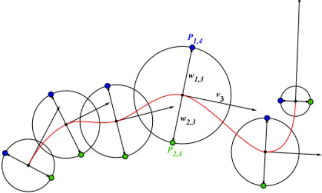
The basic idea is the following. Each circle(ci, ri)is transformed into a spatial point pi and an interpolating spatial curve from Hermite arcs is constructed to these points, where the tangents are defined by Bessel’s method. Now at each circle the spatial tangent line e of the Hermite arc has an intersection point Te with the plane of the circles, from which we draw the planar tangent lines to the given circle. This way we obtain two points, E1 and E2, which will be touching points of the future interpolation curves (see Fig. 9).
Computationally we have to determine the angle between the line connecting the center of the circle to the intersection point of the spatial tangent, and the line connecting the center to the touching points of the planar tangents. The method works well in some extraordinary situation as well, even when the planar curve driven method would fail. This frequently happens if two neighboring circles are close to each other meanwhile their radius are strongly different (Fig. 10).
4. Conclusion and further research
Localization of touching points for interpolation of given circles are discussed.
We considered two methods, which solves the problem in several cases, but none
Figure 9: Planar tangent lines to the circle are drawn from the intersection point of the plane and the tangent line of the spatial
curve. Perspective and upper view
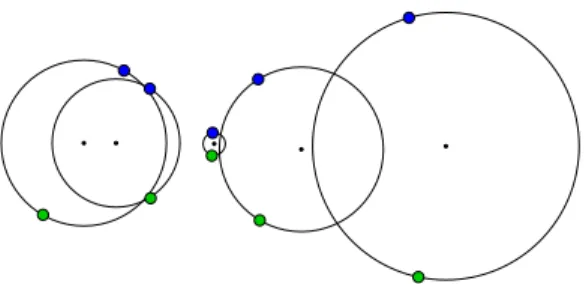
Figure 10: Spatial curve driven method gives acceptable result even in case of sudden changes of radius of neighboring circles
of them are perfect. Although the spatial curve driven method solves the problem in most cases, in extreme positions of the given circles both methods can fail, thus future improvements are required. One possibility is to change the simple Hermite interpolation by some more sophisticated methods, but we think it cannot solve the problem in general. Other geometric ways of finding touching points are under development.
References
[1] Au, C.K., Yuen, M.M.F., Unified approach to NURBS curve shape modification, Computer-Aided Design, 27 (1995), 85–93.
[2] Farin, G., Curves and Surface for Computer-Aided Geometric Design, 4th edition, Academic Press, New York, 1997.
[3] Piegl, L., Tiller, W., The NURBS book, Springer–Verlag, 1995.
[4] Hoschek, J., Lasser, D., Fundamentals of CAGD, AK Peters, Wellesley, MA, 1993.
[5] Tai, C.-L., Barsky, B.A., Loe, K.-F., An interpolation method with weight and relaxation parameters. In: Cohen, A., Rabut, C., Schumaker, L.L. (eds.): Curve and Surface Fitting: Saint-Malo 1999. Vanderbilt Univ. Press, Nashville, Tenessee, (2000), 393–402.
[6] Tai, C.-L., Wang, G.-J., Interpolation with slackness and continuity control and convexity-preservation using singular blending, J. Comp. Appl. Math., 172 (2004), 337–361.
[7] Pan, Y.-J., Wang, G.-J., Convexity-preserving interpolation of trigonometric poly- nomial curves with shape parameter,Journal of Zhejiang Univ. Sci., 8 (2007), 1199–
1209.
[8] Hoffmann, M., Juhász, I.On interpolation by spline curves with shape parame- ters,Lecture Notes in Computer Science, 4975 (2008), 205–215.
[9] Peternell, M., Odehnal, B., Sampoli, M.L.On quadratic two-parameter fami- lies of spheres and their envelopes,Comput. Aided Geom. Design25 (2008), 342–355.
[10] Slabaugh, G., Unal, G., Fang, T., Rossignac, J., Whited, B., Variational Skinning of an Ordered Set of Discrete 2D Balls,Lecture Notes on Computer Science, 4795 (2008), 450–461.
[11] Cheng, H., Shi, X., Quality mesh generation for molecular skin surfaces using restricted union of balls. Proc. IEEE Visualization Conference (VIS2005), (2005), 399–405.
[12] Edelsbrunner, H., Deformable smooth surface design,Discrete and Computational Geometry, 21 (1999), 87–115.
[13] Kruithof, N., Vegter, G., Envelope Surfaces, Proc. Annual Symposium on Com- putational Geometry, (2006), 411–421.
Roland Kunkli
Department of Computer Graphics and Image Processing University of Debrecen
H-4010 Debrecen Hungary
e-mail: rkunkli@gmail.com

![Figure 3: A good result by Slabaugh’s method (from [10])](https://thumb-eu.123doks.com/thumbv2/9dokorg/1214797.91410/3.714.221.501.284.457/figure-good-result-slabaugh-s-method.webp)