Cautionary note on calculating standardized effect size (SES) in randomization test

(1)

1585-8553 © The Author(s).

This article is published with Open Access at www.akademiai.com DOI: 10.1556/168.2018.19.1.8

Introduction

The null-hypothesis testing is a widely used statistical approach in ecology. However, it is often criticized because it allows only a dichotomous decision: reject or fail to reject the null-hypothesis. Indeed, it does not provide information re- garding the magnitude of an effect of interest (Nakagawa and Cuthill 2007). One possible way to overcome this limitation is to calculate effect size, i.e., the magnitude of an effect (e.g., mean difference from the control or between two groups).

Effect sizes can be subsequently used in a meta-analysis for a quantitative synthesis of the primary results (Harrison 2011, Koricheva et al. 2013). Furthermore, even within a study, regressing plot-level effect sizes against environmental factors can provide additional and meaningful information (e.g., Schamp and Aarssen 2009). This approach is widely used in community assembly studies (e.g., Bernard-Verdier et al.

2012, Mason et al. 2012, Astor et al. 2014, Lhotsky et al.

2016), when the strength of trait convergence/divergence was studied along an environmental gradient.

Textbooks of meta-analysis (e.g., Koricheva et al. 2013, Rothstein et al. 2013) demonstrate how test-statistics of the traditional tests (e.g., t-test, ANOVA, regression) can be transformed into an effect size measure. However, in community ecology, the use of randomization tests (Gotelli and Graves 1996) has become common because they allow the user to choose the statistic that best discriminates between the hypothesis and alternative; regardless of whether its dis-

tribution is known or not. This paper focuses on measuring effect size in studies where the randomization test is applied, which is a large and growing field within community ecology (Appendix 1). Although similar problems may appear in other applications of the meta-analysis, the proposed solution is specific to this field.

If null-hypothesis is tested by randomization test, departure from the random expectation is often measured as a standardized effect size (SES; Gotelli and McCabe 2002).

SES measures the deviation from the random expectation in standard deviation units, which allows the comparison of values between studies:

SES = (I_obs – I_rand) / s

where Iobs = the observed value of the index, Irand = the mean of the index in the random communities, σ = standard deviation of the index in the random communities (Gotelli and McCabe 2002). Alternative naming of the same formula is z-score (e.g., Heino et al. 2015, Stoll et al. 2016) or z-value (e.g., Briscoe Runquist et al. 2016). Nearest taxon index (Webb et al. 2002) and β deviation (Kraft et al. 2011, Bennett and Gilbert 2016) are special forms of SES, where the index I refers to (A) the phylogenetic distance to the nearest taxon and (B) the beta diversity, respectively.

The formula of SES can be derived from the d statistic (often referred to as Hedges' g or Cohen's d in the literature).

Observed and random values are the two groups. Because we

Cautionary note on calculating standardized effect size (SES) in randomization test

Z. Botta-Dukát

Centre for Ecological Research, Institute of Ecology and Botany, Alkotmány u. 2-4, Vácrátót, Hungary.

E-mail: botta-dukat.zoltan@okologia.mta.hu; http://www.okologia.mta.hu/en/Zoltan.BOTTA-DUKAT Keywords: Functional diversity; Randomization test; Standardized effect size; Statistics.

Abstract. In community ecology, randomization tests with problem specific test statistics (e.g., nestedness, functional diversity, etc.) are often applied. Researchers in such studies may want not only to detect the significant departure from randomness, but also to measure the effect size (i.e., the magnitude of this departure). Measuring the effect size is necessary, for instance, when the roles of different assembly forces (e.g., environmental filtering, competition) are compared among sites. The standard meth- od is to calculate standardized effect size (SES), i.e., to compute the departure from the mean of random communities divided by their standard deviations. Standardized effect size is a useful measure if the test statistic (e.g., nestedness index, phylogenetic or functional diversity) in the random communities follows a symmetric distribution. In this paper, I would like to call attention to the fact that SES may give us misleading information if the distribution is asymmetric (skewed). For symmetric distribution median and mean values are equal (i.e., SES = 0 indicates p = 0.5). However, this condition does not hold for skewed distributions.

For symmetric distributions departure from the mean shows the extremity of the value, regardless of the sign of departure, while in asymmetric distributions the same deviation can be highly probable and extremely improbable, depending on its sign. To avoid these problems, I recommend checking symmetry of null-distribution before calculating the SES value. If the distribution is skewed, I recommend either log-transformation of the test statistic, or using probit-transformed p-value as effect size measure.

Abbreviations: CDF–Cumulative Distribution Function; LDMC–Leaf Dry Matter Content; Q–Rao’s Quadratic entropy; SES–

Standardized Effect Size; SLA–Specific Leaf Area.

(2)

have only one value in the observed group, the formula for the pooled standard deviation reduces to s.

SES is widely used in community ecology because (until now) it is the only proposed way to calculate effect size when a randomization test needs to be applied. The index could be a co-occurrence based statistic (Gotelli and McCabe 2002), nestedness (Ulrich and Gotelli 2007), functional diversity (Mason et al. 2012) or any other measure that is appropriate to the studied question.

Unfortunately, most users of SES do not acknowledge that normality (or at least symmetry) of the null-distribution is required when calculating SES (Ulrich and Gotelli 2010, Veech 2012). To illustrate that the normality assumption is widely neglected, I have collected 63 papers (published since 2015 and that calculated SES; see details in Appendix 1) and assessed if such an assumption was mentioned. Only eight papers mentioned the normality assumption and seven of them assumed that normality was satisfied without testing this assumption.

Therefore, the aims of this paper are (1) to illustrate that SES values are misleading if the null-distribution is asymmetric; and (2) to show an alternative way to calculate effect size that works properly, even if the null-distribution is asymmetric (skewed).

Field data used for illustration

All illustrative examples come from the field of trait-based community assembly studies (Götzenberger et al. 2012), but their messages can be easily generalized to other fields that utilize randomization tests. The primary hypothesis of these studies is that communities are not randomly assembled from the regional species pool; therefore, their functional diversity is considerably different from the functional diversity of a random assemblage. Departure from the random expectation is possible in both directions. Co-occurring species need to survive and reproduce in the same environment; therefore, in traits related to environmental tolerance, they are more similar to each other than members of a random assemblage.

Thus, functional diversity may be lower than expected. On the other hand, according to the niche theory (MacArthur and Levins 1967, Pásztor et al. 2016), co-occurring species have to differ in resource use; therefore, they are more different in the related traits than members of a random assemblage.

Thus, functional diversity may be higher than expected. The situations when observed functional diversity is lower/higher than random expectation are referred to as trait convergence/divergence. It is not only the existence of significant departure from the random expectation (hereafter referred as significant convergence/divergence) that is informative, but also the magnitude of the departure (hereafter referred to as strength of convergence/divergence). In such studies SES is often used as a standardized measure of the departure from random expectation. Standardized means that the potential effect of the confounding factors (e.g., species richness, diversity) were removed. It is supposed that the absolute value of SES measures the strength of convergence/divergence. For

example, SES = 2 and SES = –2 are interpreted as trait divergence and trait convergence, respectively, with the same strength (and same related p-value).

The dataset used for illustration was derived from the paper of Lhotsky and colleagues (2016) and is publicly avail- able in the Dryad repository (http://datadryad.org/resource/

doi:10.5061/dryad.5r62f). In this example, I considered only five quantitative traits: canopy height, leaf size, specific leaf area (SLA), leaf dry matter content (LDMC) and seed weight. Two functional diversity indices were used to quan- tify trait convergence or divergence: Rao's quadratic entropy, Q (Botta-Dukát 2005) and generalized functional diversity, with q = 2, ²D (Leinster and Cobbold 2011). Rao's quadratic entropy was chosen because it is a widely used measure of functional diversity. ²D is a simple, monotonic transforma- tion of Rao's Q:

2D = 1 / (1 – Q)

2D is advantageous because it allows for the partitioning of gamma diversity into independent alpha and beta components (Leinster and Cobbold 2011, Botta-Dukát 2018). A randomization test was done by reshuffling trait values among species (Stubbs and Wilson 2004, Botta-Dukát and Czúcz 2016). Test statistics and effect sizes were calculated for each plot separately.

The problem

As discussed above, SES was developed under the assumption of Gaussian distribution of test statistic if the null- hypothesis is true. If the normality assumption is valid, SES values and the cumulative distribution function (CDF) of the standard normal distribution (hereafter denoted by F) can be used to calculate p-values, instead of the cumulative distribution function of the test statistic (see its mathematical background in Appendix 2). The advantage of calculating the p-value from SES instead of the empirical CDF is that an accurate estimation of CDF requires a much larger sample size (i.e., more randomized communities) than the accurate estimation of expected value and standard deviation (the parameters of the normal distribution). It is obvious that p-values calculated from SES are valid only if the null-distribution ap- proximates to a Gaussian. Figure 3 of Veech (2012) illustrates that if the normality assumption is violated, the estimate of the p-value based on SES may be strongly biased and results in increased Type I error or decreased power of the test.

The assumption of normality and symmetry is intermixed in the literature. For example, Ulrich and Gotelli (2010) wrote: "The use of SES is based on the assumption of an ap- proximately normal error distribution. This was indeed the case: the mean skewness of all null-model distributions was only 0.004 with a standard deviation of 0.37". They mention normal distribution; however, by calculating skewness they have checked only for symmetry of the distribution. The null- distribution may be symmetric, even if it significantly departs from normal distribution (e.g., the uniform distribution is symmetric). In this case SES values cannot be used for hy-

(3)

pothesis testing, but they are useful as measure of departure from the random expectation. However, if the null-distribution is asymmetric (skewed), SES values become misleading.

For symmetric distributions – including Gaussian distribution – cumulative distribution function (CDF) is 0.5 at the expected value (mean), that is in a one-sided test the corresponding p-value is 0.5 too. I_rand is an unbiased estimate of the expected value. Therefore, SES = 0 implies that a one-sided p-value is 0.5 if the distribution is symmetric (Fig. 1a). Moreover, the absolute value of the SES determines the p-value of the two-sided test.

These relationships are not maintained in skewed distributions, i.e., the mean is higher or lower than the median in the right or left skewed distribution, respectively. Therefore,

SES values that differ only in sign may be related to markedly different p-values (Fig. 1b).

Figure 2 shows a real data example that illustrates the problem originating from the violation of the symmetry assumption. As mentioned above, SES = 2 and SES = –2 should indicate the same strength of trait divergence or convergence, respectively. In the fi gure whiskers indicate the range of non- signifi cant SES values in a two-sided test when signifi cance level is 5% (α = 0.05). SES = –2 is outside the non-signifi cant region and is far from the border of the region in all communities. Thus, this value indicates strong and signifi cant trait convergence. On the other hand, SES = 2 (i.e., the same absolute effect size, but with opposite sign) is often non-signifi - cant (i.e., it is inside the whiskers), and even if signifi cant this happens near the border of the non-signifi cant region. Thus,

Figure 1. Position of three standardized effect size (SES) values (-2, 0, 2) and the related p-values in two-sided tests for (a) a symmetric (normal) and (b) right skewed (lognormal) distribution.

a b

Figure 2. Whiskers plots indicate the range of non-signifi cant SES values in two sided tests at α = 5% signifi cance levels (i.e., borders of the region are 2.5% and 97.5% quantiles of the null-distribution) in the fi rst 25 communities from a dataset reported in Lhotsky et al. (2016). The applied test statistic was functional diversity based on leaf size data calculated by ²D. For symmetric null-distribution whiskers would be placed symmetrically around the zero-line. Due to right skewness, the same absolute value with a negative sign may reveal highly signifi cant trait convergence, while the positive sign may indicate no signifi cant departure from randomness.

Figure 2. Whiskers plots indicate the range of non-significant SES values in two sided tests at

= 5% significance levels (i.e. borders of the region are 2.5% and 97.5% quantiles of the

null-distribution) in the first 25 communities from a dataset reported in Lhotsky et al. (2016).

The applied test statistic was functional diversity based on leaf size data calculated by

²

D. For symmetric null-distribution whiskers would be placed symmetrically around the zero-line.

Due to right skewness, the same absolute value with a negative sign may reveal highly significant trait convergence, while the positive sign may indicate no significant departure from randomness.

b

(4)

it indicates weak and often non-significant trait divergence.

In this example, comparing the strength of trait convergence and trait divergence measured by SES would be misleading.

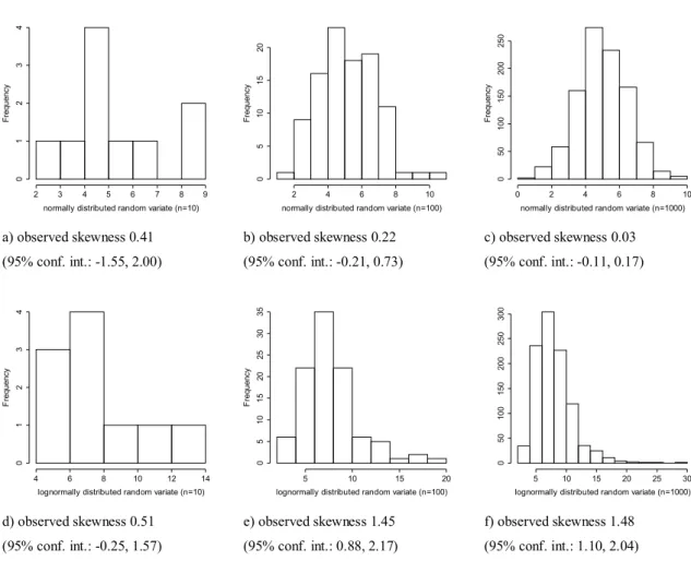
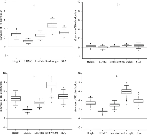
Symmetry of distribution can be visually checked using histograms of values in random communities, although for small number of random communities it cannot lead to a reliable decision (Fig. 3). Therefore, I suggest estimating skewness from data (possible estimators are reviewed by Joanes and Gill 1998). Symmetry has to be checked for each null-distribution separately. Therefore, if the number of null-distributions that are generated is high, estimating skewness is the only feasible option. Information of the calculated skewness values can be summarized using a boxplot (Fig. 4).

Possible solutions

Two possible ways to avoid the above mentioned draw- backs of SES are to apply a transformed test statistic and to use probit-transformed p-values to measure effect size. Any monotonous transformation of the test statistic that considerably decreases the skewness may be applied. Unfortunately, there is no generally applicable transformation that can re- duce the skewness to an acceptable level in all instances. If the distribution is right skewed, a log-transformation is often

applied. Figure 4 illustrates that the log-transformation may be effective in some cases but ineffective in others.

As mentioned above, under the assumption of Gaussian null-distribution, p-values can be calculated from SES by applying the cumulative distribution function of the standard normal distribution (F). For example, in a one-sided test of trait convergence p-values can be estimated as 1 – F (SES) (see Appendix 2 for the deduction of this formula and for- mulae for a one-sided test of divergence and two-sided test).

This approach is used by Sanders et al. (2003), Schamp and Aarssen (2009), or de Bello (2012).

In randomization tests, p-values are generally estimated using a direct approach (Veech, 2012) as:

p = (b + 1) / (n + 1)

where n = number of random communities, b = number of random communities, where the test statistic is more extreme than the observed value (e.g., Manly 1997). This estimation does not assume any specific distribution. Thus, if the null- distribution is not Gaussian we know the p-value but do not know the effect size (in this case, SES calculated by Gotelli and Grave's formula is not suitable). We are looking for an effect size measure (denoted by ES) that is equal to SES if a) observed skewness 0.41

(95% conf. int.: -1.55, 2.00)

b) observed skewness 0.22 (95% conf. int.: -0.21, 0.73)

c) observed skewness 0.03 (95% conf. int.: -0.11, 0.17)

d) observed skewness 0.51 (95% conf. int.: -0.25, 1.57)

e) observed skewness 1.45 (95% conf. int.: 0.88, 2.17)

f) observed skewness 1.48 (95% conf. int.: 1.10, 2.04)

326 Figure 3: Histograms and estimated skewness with 95% confidence intervals in brackets for 327

normally (a-c) and lognormally (d-f) distributed random numbers with different sample sizes 328

(n). Parameters of both distributions were set to an expected value = 8 and standard deviation 329

= 3. Skewness values were estimated using the Skew function of DescTools package 330

(Signorell 2015) in R environment (R Core Team, 2013) 331

332

normally distributed random variate (n=10)

Frequency

2 3 4 5 6 7 8 9

01234

Frequency

2 4 6 8 10

05101520

Frequency

0 2 4 6 8 10

050100150200250

lognormally distributed random variate (n=10)

Frequency

4 6 8 10 12 14

01234

Frequency

5 10 15 20

05101520253035

5 10 15 20 25 30

050100150200250300

Figure 3. Histograms and estimated skewness with 95% confidence intervals in brackets for normally (a-c) and lognormally (d-f) distributed random numbers with different sample sizes (n). Parameters of both distributions were set to an expected value = 8 and standard deviation = 3. Skewness values were estimated using the Skew function of DescTools package (Signorell 2015) in R environment (R Core Team, 2013)

(5)

the normality assumption is satisfied, while preserving the advantages of SES if this assumption is violated. I suggest that we can find such an ES using two simple steps. First, recall the formula used in calculating p-value from SES, but replace SES with the desired ES: p = 1–F (ES). Then we can solve this equation for ES: ES = F^–1(1 – p). F^–1 is the inverse of F, thus F^–1 is the quantile function of the standard normal distribution. It is often called a probit-function, or probit- transformation. Hereafter I will use this name and abbreviate it by probit(1-p).

There are two advantages of SES over probit(1-p): the former is less sensitive to the number of random communities. If the normality criterion is satisfied, SES gives an accurate estimation of the effect size even if only a few random communities are generated. An additional important advantage of SES is that it is unbounded. Thus, it can differentiate even between large effect sizes. Using a traditional approach, the lowest p-value, and consequently the highest probit(1- p) depends on the number of generated random communi- ties. The possible minimum of p is 1/(n+1) (c.f. formula for

calculating p above). Thus, it is possible that two estimated probit(1-p) may be the same simply because both equal the possible maximum. Knijnenburg et al. (2009) provided a solution to this problem. Their approach allows exact estimation of p-values, even if the observed value is more extreme than any value in the random communities. The suggested procedure consists of two steps: fitting generalized Pareto- distribution of the most extreme random values and then estimating p-values from this fitted distribution (See Appendix 3 for an R-script of this procedure).

Conclusions

As shown above, SES calculated by Gotelli and McCabe's (2002) formula is misleading if the symmetry assumption is violated. Because this assumption is hardly tested, results based on SES values should be carefully considered. It is also true for p-values or significance tests based on SES where not only symmetry but normality of the null-distribution is assumed.

Figure 4. Skewness of distribution of functional diversity in random communities using four different test statistics: a) generalized functional diversity with q = 2 (

²D); b) log-transformed

2D; c) Rao’s quadratic entropy (Q); d) log-transformed Q. Random communities were

generated by reshuffling trait values for 103 plots of Lhotsky et al. (2016) resulting in 103 skewness values.

Figure 4. Skewness of distribution of functional diversity in random communities using four different test statistics: a) generalized functional diversity with q = 2 (2D); b) log-transformed 2D; c) Rao’s quadratic entropy (Q); d) log-transformed Q. Random communities were generated by reshuffling trait values for 103 plots of Lhotsky et al. (2016) resulting in 103 skewness values.

a b

c d

(6)

To avoid such errors, I recommend checking at minimum the symmetry of the null-distribution. However, if SES is used to calculate p-values or to determine statistical significance, normality should also be tested. If the symmetry assumption is violated, one can attempt to solve it using a log-transformation of the test statistic. However, log-transformations cannot solve this problem in all cases, thus the null-distribution of transformed values will need to be checked again. An alternative solution proposed in this paper is to use probit(1-p) as an effect size measure, where p-values are estimated using an algorithm found in Knijnenburg et al. (2009). If the normality assumption is satisfied, it results in the same value as SES, thus effect sizes calculated in this way are comparable with the published SES values.

Acknowledgement. Thanks to M. Scotti, B. Lhotsky and two anonymous reviewers for their comments that helped to im- prove the manuscript.

References

Astor, T., J. Strengbom, M.P. Berg, L. Lenoir, B. Marteinsdóttir and J. Bengtsson. 2014. Underdispersion and overdispersion of traits in terrestrial snail communities on islands. Ecol. Evol. 4:2090–

2102.

de Bello, F. 2012. The quest for trait convergence and divergence in community assembly: are null-models the magic wand? Global Ecol. Biogeogr. 21:312–317.

Bennett, J. R. and B. Gilbert. 2016. Contrasting beta diversity among regions: how do classical and multivariate approaches compare?

Global Ecol. Biogeogr. 25:368–377.

Bernard-Verdier, M., M.-L. Navas, M. Vellend, C. Violle, A. Fayolle and E. Garnier. 2012. Community assembly along a soil depth gradient: contrasting patterns of plant trait convergence and divergence in a Mediterranean rangeland. J. Ecol. 100:1422–1433.

Botta-Dukát, Z. 2005. Rao’s quadratic entropy as a measure of functional diversity based on multiple traits. J. Veg. Sci. 16:533–540.

Botta-Dukát, Z. 2018. The generalized replication principle and the partitioning of functional diversity into independent alpha and beta components. Ecography 41:40–50.

Botta-Dukát, Z. and B. Czúcz. 2016. Testing the ability of functional diversity indices to detect trait convergence and divergence using individual-based simulation. Methods Ecol. Evol. 7:114–126.

Briscoe Runquist, R., D. Grossenbacher, S. Porter, K. Kay and J.

Smith. 2016. Pollinator-mediated assemblage processes in California wildflowers. J. Evol. Biol. 29:1045–1058.

Gotelli, N.J. and G.R. Graves. 1996. Null Models in Ecology.

Smithsonian Institution Press, Washington, D.C.

Gotelli, N.J. and D.J. McCabe. 2002. Species co-occurrence: a meta-analysis of J. M. Diamond’s assembly rules model. Ecology 83:2091–2096.

Götzenberger, L., F. de Bello, K.A. Bråthen, J. Davison, A. Dubuis, A.

Guisan, J. Lepš, R. Lindborg, M. Moora, M. Pärtel, L. Pellissier, J. Pottier, P. Vittoz, K. Zobel and M. Zobel. 2012. Ecological assembly rules in plant communities—approaches, patterns and prospects. Biol. Rev. 87:111–127.

Harrison, F. 2011. Getting started with meta-analysis. Methods Ecol.

Evol. 2: 1–10.

Heino, J., J. Soininen, J. Alahuhta, J. Lappalainen and R. Virtanen.

2015. A comparative analysis of metacommunity types in the freshwater realm. Ecol. Evol. 5:1525–1537.

Joanes, D.N. and C.A. Gill. 1998. Comparing measures of sample skewness and kurtosis. J. Roy. Stat. Soc. D 47:183–189.

Knijnenburg, T.A., L.F.A. Wessels, M.J.T. Reinders and I. Shmu levich. 2009. Fewer permutations, more accurate P-values.

Bioinformatics 25:i161–i168.

Koricheva, J., J. Gurevitch and K. Mengersen (eds.) 2013. Handbook of Meta-analysis in Ecology and Evolution. Princeton University Press, Princeton.

Kraft, N.J.B., L.S. Comita, J.M. Chase, N.J. Sanders, N.G. Swenson, T.O. Crist, J.C. Stegen, M. Vellend, B. Boyle, M.J. Anderson, H.V. Cornell, K.F. Davies, A.L. Freestone, B.D. Inouye, S.P.

Harrison and J.A. Myers. 2011. Disentangling the drivers of β diversity along latitudinal and elevational gradients. Science 333:1755–1758.

Leinster, T. and C.A. Cobbold. 2011. Measuring diversity: the impor- tance of species similarity. Ecology 93:477–489.

Lhotsky, B., B. Kovács, G. Ónodi, A. Csecserits, T. Rédei, A.

Lengyel, M. Kertész and Z. Botta-Dukát. 2016. Changes in assembly rules along a stress gradient from open dry grasslands to wetlands. J. Ecol. 104:507–517.

MacArthur, R. and R. Levins. 1967. The limiting similarity, convergence, and divergence of coexisting species. Amer.Nat.

101:377–385.

Manly, B.F.J. 1997. Randomization, Bootstrap and Monte Carlo Methods in Biology. Second Edition. Chapman & Hall, London.

Mason, N.W.H., S.J. Richardson, D.A. Peltzer, F. de Bello, D.A.

Wardle and R.B. Allen. 2012. Changes in coexistence mecha- nisms along a long-term soil chronosequence revealed by functional trait diversity. J. Ecol. 100:678–689.

Nakagawa, S. and I.C. Cuthill. 2007. Effect size, confidence interval and statistical significance: a practical guide for biologists. Biol.

Rev. 82:591–605.

Pásztor, E., Z. Botta-Dukát, T. Czárán, G. Magyar and G. Meszéna.

2016. Theory Based Ecology. The Darwinian Approach. Oxford Uninersity Press, Oxford, UK.

R Core Team. 2013. R: A language and environment for statistical computing. R Foundation for Statistical Computing, Vienna, Austria. URL: http://www.R-project.org

Rothstein, H., M. Borenstein, L.V. Hedges and J.P.T. Higgins. 2013.

Introduction to Meta-analysis. Wiley, Hoboken, N.J.

Sanders, N.J., N.J. Gotelli, N.E. Heller and D.M. Gordon. 2003.

Community disassembly by an invasive species. PNAS 100:2474–2477.

Schamp, B.S. and L. W. Aarssen. 2009. The assembly of forest communities according to maximum species height along resource and disturbance gradients. Oikos 118:564–572.

Signorell, A. 2015. DescTools: Tools for descriptive statistics.

Stoll, S., P. Breyer, J.D. Tonkin, D. Früh and P. Haase. 2016. Scale- dependent effects of river habitat quality on benthic invertebrate communities — Implications for stream restoration practice. Sci.

Total Env. 553:495–503.

Stubbs, W.J. and J.B. Wilson. 2004. Evidence for limiting similarity in a sand dune community. J. Ecol. 92:557–567.

Ulrich, W. and N.J. Gotelli. 2007. Null model analysis of species nestedness patterns. Ecology 88:1824–1831.

Ulrich, W. and N.J. Gotelli. 2010. Null model analysis of species as- sociations using abundance data. Ecology 91:3384–3397.

(7)

Veech, J. A. 2012. Significance testing in ecological null models.

Theor. Ecol. 5:611–616.

Webb, C.O., D.D. Ackerly, M.A. McPeek and M.J. Donoghue. 2002.

Phylogenies and community ecology. Annu. Rev. Ecol. Syst.

33:475–505.

Received September 15, 2017 Revised December 31, 2017, March 28, May 24, 2018 Accepted May 30, 2018

Appendices

Appendix 1: Data on papers using SES

Appendix 2: The relationship of SES and p-values when normality assumption is satisfied

Appendix 3: R function for calculating p-values applying ap- proach Knijnenburg et al. 2009

The Appendices may be downloaded from www.akademiai.

com.

Open Access. This article is distributed under the terms of the Creative Commons Attribution 4.0 International License (https://creativecommons.org/licenses/by/4.0/), which permits unrestricted use, distribution, and reproduction in any medium, provided the original author and source are credited, you give a link to the Creative Commons License, and indicate if changes were made.