arXiv:1608.05237v2 [math.CO] 11 Oct 2016
TRIANGLE-DIFFERENT HAMILTONIAN PATHS
ISTV ´AN KOV ´ACS AND DANIEL SOLT´ESZ
Abstract. LetGbe a fixed graph. Two paths of lengthn−1 onnvertices (Hamiltonian paths) areG-different if there is a subgraph isomorphic toGin their union. In this paper we prove that the maximal number of pairwise triangle-different Hamiltonian paths is equal to the number of balanced bipartitions of the ground set, answering a question of K¨orner, Messuti and Simonyi.
1. Introduction
Problems concerning the size of largest sets of permutations pairwise satisfying a pre- scribed relation has a large literature, see e.g. [6, 7]. Investigations of a special type of such problems related to the Shannon capacity of infinite graphs, a notion analo- gous to Shannon’s graph capacity concept, was initiated in [8]. Two permutations π1, π2
of [n] := {1, . . . , n} are called colliding in [8] if there is an index i ∈ [n] such that
|π1(i)−π2(i)|= 1.
Conjecture 1.1 (K¨orner, Malvenuto). [8] The maximal number of pairwise colliding permutations of [n] is ⌊nn2⌋
. In Conjecture 1.1 ⌊nn2⌋
is best possible, since permutations containing numbers of the same parity at every position do not collide, so the maximal number of pairwise colliding permutations is at most the number of ”parity patterns”, that is, the number of ways ⌈n2⌉ odd and⌊n2⌋even numbers can be placed onn positions if only the parity of the numbers matter, their actual value do not. The largest construction known contains roughly 1.81n permutations (see [2]). Conjecture 1.1 triggered the investigation of several problems of the same flavor that concern the maximal number of permutations any pair of which satisfy some specified constraint, see [2, 9, 13]. There is a natural relationship between Hamiltonian paths and permutations. In this paper we focus on problems of the above type that can naturally be formulated in terms of Hamiltonian paths.
The union of two graphsH1 andH2 on the same vertex set is the graph on this common vertex set having E(H1)∪E(H2) as edge set. Let G be some fixed graph. We say that two Hamiltonian paths are G-different if their union contains G as a subgraph. The maximal number of pairwise G-different Hamiltonian paths has been studied for various Gin [4, 10, 11]. The problem is uninteresting when Gis contained in a Hamiltonian path.
(The maximal size of G-different families in these cases is simply n!2.) A somewhat more interesting case is that of K1,3-different Hamiltonian paths. It is easy to see that the union of two Hamiltonian paths does not contain a vertex of degree 3 if and only if the union itself is a Hamiltonian cycle. Thus the maximal size of K1,3-different Hamiltonian paths is (n−1)!2 . The first few choices forG, where the problem becomes more difficult, are:
K3, K4, C4, K1,4. Until now even the correct order of magnitude was unknown for these
The research of the first author was supported by National Research, Development and Innovation Office NKFIH, K-111827.
The research of the second author was supported by the Hungarian Foundation for Scientific Research Grant (OTKA) No. 108947.
1
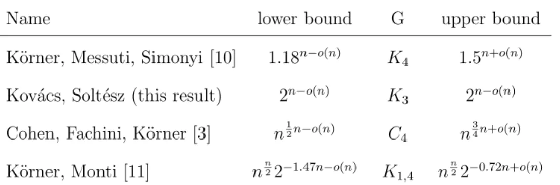
families, for the best lower and upper bounds known so far see Table 1. In this paper we determine the maximal number of pairwise triangle-different Hamiltonian paths onn vertices exactly.
K¨orner, Messuti and Simonyi made the following observation.
Proposition 1.2. [10] The maximal number of Hamiltonian paths such that every pair- wise union contains an odd cycle is equal to the number of balanced bipartitions of the vertex set. That is, on 2n+ 1 vertices this number is 2n+1n
and on 2n+ 2 vertices it is
1 2
2n+2 n+1
= 2n+1n .
The upper bound follows by observing that a Hamiltonian path is a bipartite graph with a balanced bipartition and the union of two paths with the same bipartition is a bipartite graph which clearly cannot contain any odd cycle. On the other hand, if for every balanced bipartition we choose an arbitrary Hamiltonian path that corresponds to it, then we obtain a good family.
The authors in [10] asked whether the same upper bound can be attained with pairwise triangle-different Hamiltonian paths. They verified that this is possible up to 5 vertices.
By an easy product construction this yields a lower bound of roughly 1.58n.
An affirmative answer to the above question may be interpreted by saying that insist- ing on a triangle in the pairwise unions is not more restrictive than requiring just any odd cycle. As noted in [10], there are some famous theorems of this kind that show the indifference of specifying the triangle among odd cycles in certain situations. For exam- ple, the maximum number of edges in an odd-cycle-free (bipartite) graph isj
n2 4
k and the Mantel-Tur´an theorem states that this number is the same for triangle-free graphs. An- other slightly related example is the following celebrated theorem, where the authors are interested in the intersection of general graphs instead of unions of Hamiltonian paths.
Theorem 1.3 (D. Ellis, Y. Filmus, E. Friedgut [5]). The following three numbers are equal.
• The maximum number of n-vertex graphs such that every pairwise intersection contains an odd cycle.
• The maximum number of n-vertex graphs such that every pairwise intersection contains a triangle.
• The number of n-vertex graphs that contain a fixed triangle.
We will show that the union version of Theorem 1.3 is much easier in Section 4. The main result of the present paper is the following theorem which answers the question of K¨orner, Messuti and Simonyi affirmatively.
Theorem 1.4. The maximum number of Hamiltonian paths such that every pairwise union contains a triangle is equal to the number of balanced bipartitions of the ground set.
Since the same upper bound holds as in Proposition 1.2, the main challenge is to construct a family of this size that satisfies the condition.
We prove Theorem 1.4 in Section 2. In Section 3 we also investigate the case one can consider the ”other extreme”, where we look for large families of Hamiltonian paths any two of which forming a union that contains a Hamiltonian cycle. We prove that the maximal number of such Hamiltonian-cycle-different Hamiltonian paths on n vertices is at most n2
and provide a construction which achieves this bound whenever n is prime.
Section 5 contains some open problems and concluding remarks.
2
Name lower bound G upper bound K¨orner, Messuti, Simonyi [10] 1.18n−o(n) K4 1.5n+o(n) Kov´acs, Solt´esz (this result) 2n−o(n) K3 2n−o(n) Cohen, Fachini, K¨orner [3] n12n−o(n) C4 n34n+o(n) K¨orner, Monti [11] nn22−1.47n−o(n) K1,4 nn22−0.72n+o(n) Table 1. The order of magnitude of the lower and upper bounds for the maximal size of pairwise G-different Hamiltonian paths for the first few non-trivial choices for G.
2. Proof of the main theorem
In this section we prove Theorem 1.4. The number of balanced bipartitions of 2n+ 1 and 2n + 2 vertices is the same, namely 2n+1n
. Thus it is enough to construct 2n+1n triangle-different Hamiltonian paths on 2n+ 1 vertices, since we can add an additional vertex and extend every original Hamiltonian path by an edge when we want a good construction of the same size on 2n+ 2 vertices. We say that two Hamiltonian paths are compatible if their union contains a triangle. We also say that a set of Hamiltonian paths is compatible if each pair of them is compatible. We will construct a compatible set of Hamiltonian paths of the required size. Within our construction the Hamiltonian paths will belong to several groups (called types) according to the following definition.
Definition 2.1. Let G be a graph with weighted edges where the weights are 1 or 2. We say that a Hamiltonian path H on the vertex set of G is G-type if the following holds.
For every u and v that are connected in G by an edge of weight w, the distance of u and v in H is exactly w.
By weighted graph we will always mean a weighted graph where the edges get weight 1 or 2. When drawing a weighted graph we will draw the edges of weight 1 as ordinary lines, and the edges of weight 2 by dashed lines. See Figure 1 for an illustration of Definition 2.1.
x1 x2
x3
x4
x5
G1
x1 x2
x3
x4
x5
H1
x1 x2
x3
x4
x5
H2
Figure 1. Both H1 and H2 are G1-type.
Observe that ifG1 and G2 are weighted graphs that share an edge that has a different weight in G1 and in G2, then every G1-type Hamiltonian path is compatible with every G2-type Hamiltonian path. Hence we define compatibility for weighted graphs too.
Definition 2.2. Two weighted graphsG1 andG2 are compatible if they share an edge that has different weight inG1 and G2. We say that a family of weighted graphs is compatible if every pair of weighted graphs from the family is compatible.
3
Our strategy is to first build a compatible family of weighted graphs on a ground set of odd size. Then for each weighted graphGi in the family construct a set of compatible Hamiltonian paths that are Gi-type. To obtain what we want, we need that we build a suitable family so that we can construct enough Hamiltonian paths from it.
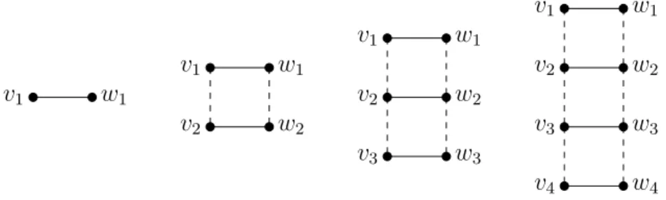
Definition 2.3. A k-ladder is a weighted graph on the vertices {v1, . . . , vk, w1, . . . , wk} where the edges of weight 1 are {(v1, w1), . . . ,(vk, wk)} and the edges of weight 2 are {(v1, v2),(v2, v3), . . . ,(vk−1, vk),(w1, w2),(w2, w3), . . . ,(wk−1, wk)}. We say that a weighted graph is a (weighted) ladder if it is a k-ladder for some k, see Figure 2. We also call the vertices (v1, w1) and (vk, wk) the top and the bottom of the ladder respectively, and we assume that for each ladder it is fixed which one of its edges is the top and which is the bottom.
We remark that we do not introduce any notation for distinguishing the top and bottom of ladders except for drawing the ladders this way on the figures.
v1 w1
v1 w1
v2 w2
v1 v2
v3
w1 w2
w3
v1
v2
v3
v4
w1
w2
w3
w4
Figure 2. k-ladders fork = 0,1,2,3. The edge (v1, w1) is the top of each ladder.
Now we define a special class of weighted graphs.
Definition 2.4. We call a weighted graph properly laddered if it is the disjoint union of ladders, an isolated vertex called the apex, and a so called residual part. This residual part can either be an empty graph, a single edge or the union of two vertex-disjoint paths on m+ 2 and m vertices, respectively, for some positive integer m. All the edges in the residual part get weight 2.
x1 x2 x3
x4 x5
x6 x7
x8 x9
x10
x11
x12
x13
x14
x15
Figure 3. A properly laddered weighted graph. The apex is x1 and the subgraph spanned by the vertices x10, x11, x12, x13, x14, x15 is the residual part.
From now on every weighted graph that we use will be properly laddered. The proof of the next Lemma describes a construction we will use to convert a properly laddered weighted graph to a set of compatible Hamiltonian paths. We will refer to this construction as the Z-swapping construction.
4
Lemma 2.5 (Z-swapping construction). LetG be a properly laddered weighted graph and let l denote the number of ladders inG. There is a set of 2l compatible Hamiltonian paths which are all G-type.
Proof. We construct a set of 2l compatible G-type Hamiltonian paths. (For simplicity we may think about our Hamiltonian paths as if they were oriented to make the term
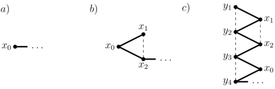
”start” of the path more appropriate. We do not really need to deal with directed edges, however.) Let us denote the apex of G by x0. Each of our Hamiltonian paths starts at the same vertex (that may or may not bex0 according to the rules below). We have three cases depending on the size of the residual part of G.
a) If the residual part of G is empty, every path starts from the apexx0.
b) If the residual part ofGconsists of a single edge (x1, x2), then every Hamiltonian path starts with the path x1x0x2.
c) If the residual part of G consists of the two paths x1. . . xm and y1. . . ym+2 then each Hamiltonian path starts with the pathy1x1y2x2. . . ymxmym+1x0ym+2. See Figure 4 for an illustration of the above cases.
x0
a)
. . . x0
x1
x2
b)
. . .
y1
y2
y3
y4
x1
x2
x0
c)
. . .
Figure 4. The shared edges of the Hamiltonian paths according to the residual part ofG.
Let R be the subgraph of G induced by the residual part and the apex. Observe that the already constructed parts of the Hamiltonian paths are R-type.
Now we direct our attention to the ladders of G. Fix an ordering of the ladders. We construct Hamiltonian paths that correspond to 0−1 sequences of length l. Each Hamil- tonian path visits (contains the weight 1 edges of) the ladders in the prescribed order.
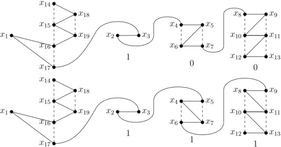
(When a Hamiltonian path visits a ladder it will traverse all its weight 1 edges before visiting the next ladder.) When a Hamiltonian path visits the ith ladder on the vertices {v1i, . . . , vkii, wi1, . . . , wkii} where the top of the ladder is the pair (v1i, wi1), it chooses from two possible paths: v1iw1iv2iw2i. . . vkiiwkii or w1iv1iw2iv2i. . . , wkivkii according to the ith coor- dinate of the 0−1 sequence, see Figure 5 (where the single indexed xj’s represent the vertices vri and wri).
Clearly, every Hamiltonian path constructed this way is G-type. These Hamiltonian paths are compatible: For two such Hamiltonian paths, letibe the first coordinate where their 0−1 sequences differ. Until the bottom of the (i−1)th ladder the two paths consist of the same edges. There is a triangle that consists of the last vertex of the paths at the bottom of the (i−1)th ladder and the two vertices at the top of the ith ladder (see Figure 5). Thus we have constructed as many pairwise compatible G-type Hamiltonian paths as many different 0−1 sequences of length l exist and this completes the proof.
Remark. Although we will not need this, we mention that it is not hard to prove that the size 2l in Lemma 2.5 is best possible. Here is a sketch of the proof. A Hamiltonian path
5
x1
x14
x15
x16
x17
x18
x19 x2 x3
1
x4 x5
x6 x7
0 0
x8 x10
x12
x9 x11
x13
x1
x14
x15
x16
x17
x18
x19 x2 x3
1
x4 x5
x6 x7
1 1
x8 x10
x12
x9 x11
x13
Figure 5. The paths that satisfy a ladder contain many parts that resem- ble a ”Z” or a reversed ”Z” shape, according to the choice made at the top, hence the name Z-swapping construction.
is a bipartite graph. Observe that the vertices on one side of a ladder must be on the same side of the bipartition, and the vertices on the other side of the same ladder must be on the other side of the bipartition. Since a Hamiltonian path is a balanced bipartite graph, the vertices of the residual part must be distributed in such a way, that the longer path is on one side, and the shorter path plus the apex is on the other, this distinguishes one side of the bipartition. Thus our only possibility to construct G-type Hamiltonian paths for a properly laddered G with different bipartitions is to ”swap” the sides of the ladders between the sides of the bipartition. Which is exactly what happens in the proof of Lemma 2.5.
For a weighted graphG, we refer to the construction of Hamiltonian paths in Lemma 2.5 as applying the Z-swapping construction toG. We also apply the Z-swapping construction to a family of weighted graphs and by this we mean that we apply it to each weighted graph in the family and we take the union of the resulting sets of compatible Hamiltonian paths.
Now we already know how to construct Hamiltonian paths from weighted graphs, thus we are left with the task of building a compatible family of weighted graphs from which we can construct the right number of Hamiltonian paths. From now on we will mainly work with weighted graphs.
Definition 2.6. We say that a compatible family F of properly laddered weighted graphs on 2n+ 1 vertices is H-maximal if applying the Z-swapping construction to F we get
2n+1 n
Hamiltonian paths.
Thus we can get the maximum possible number of Hamiltonian paths from a H-maximal family using the Z-swapping construction. Our goal is to build H-maximal families. To do this we define a similar family which satisfies an additional condition.
Definition 2.7. We say that a compatible family F of properly laddered weighted graphs on a ground set of size 2k+ 1 is MH-maximal if there is a matching M of size k that is contained in every weighted graph in F, such that every edge of M gets weight 2 in every
6
weighted graph and applying the Z-swapping construction to F we get ⌊kk2⌋
Hamiltonian paths.
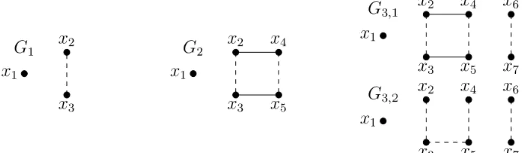
Finding MH-maximal families for small vertex sets is not difficult, see Figure 6, but it is nontrivial whether they exist for all odd-element vertex sets. (We will prove that they do in Lemma 2.9.)
x1
x2
x3
G1
x1
x2
x3
x4
x5
G2
x1
x2
x3
x4
x5
x6
x7
G3,1
x1
x2
x3
x4
x5
x6
x7
G3,2
Figure 6. For k = 1,2 an MH-maximal family consists of a single weighted graph: G1 and G2 where M is {(x2, x3)} and {(x2, x3),(x4, x5)}
respectively. Fork = 3 the weighted graphsG3,1, G3,2 form an MH-maximal family where the matching M is{(x2, x3),(x4, x5),(x6, x7)}.
Remark. Let F be an MH-maximal family on 2k + 1 vertices with the corresponding matching M. Observe that every Hamiltonian path that the Z-swapping construction produces from F is M-type. It can be proven that the maximal possible number of M- type Hamiltonian paths is also ⌊kk2⌋
, hence the name MH-maximal. Since we will not use this fact, we only sketch the argument. Hamiltonian paths are balanced bipartite graphs.
Observe that two vertices that are connected by an edge of weight two in a weighted graph G must be on the same side of the bipartition for a G-type Hamiltonian path.
Thus the vertices that are connected by an edge of M are ”glued together” so we are essentially interested in balanced bipartitions on|M|=k vertices.
The following lemma states that we can build H-maximal families using MH-maximal ones.
Lemma 2.8. If there exist MH-maximal families on ground sets of size 3,5, . . . ,2n+ 1 then there is a H-maximal family F on a ground set of size 2n+ 1.
Proof. Let the ground set be {x1, x2, . . . , x2n+1} and B be the matching that consists of the edges (x2, x3),(x4, x5), . . . ,(x2n, x2n+1). For each submatching M ⊆ B, we define a family FM of properly laddered weighted graphs as follows. We put an MH-maximal family on the vertices of M and the vertex x1 using M as the corresponding matching in the MH-maximal family and x1 as the apex. Then we extend every graph of this MH- maximal family by adding the edges of B \M with weight 1. Note that a single edge of weight 1 is a special ladder (a 1-ladder, in particular), thus FM consists of properly laddered weighted graphs. Now let
F = [
M⊆B
FM. We will prove that F is a H-maximal family.
The graphs in the family F are compatible by the following argument. Two graphs that correspond to different submatchings M1, M2 are compatible, since they contain
7
every edge in the symmetric difference M1△M2 with different weights. Two graphs that correspond to the same matching are compatible, since they are built from an MH- maximal family which consists of compatible weighted graphs.
We show that we get the desired number of Hamiltonian paths by applying the Z- swapping construction to F. First we count the number of Hamiltonian paths that we can construct from each FM. Let |M| = k, the graphs in FM are constructed from an MH-maximal family on a ground set of size 2k + 1 by adding exactly n−k edges (as 1-ladders) to every graph. By definition we get ⌊kk2⌋
Hamiltonian paths when applying the Z-swapping construction to an MH-maximal family. Since each graph in FM has n−k additional ladders, by Lemma 2.5, we get exactly ⌊kk2⌋
2n−k Hamiltonian paths by applying the Z-swapping construction toFM. Thus applying the Z-swapping construction toF, we can get exactly
n
X
k=0
n k
k k
2
2n−k
Hamiltonian paths. We are left with the task of proving the following combinatorial identity:
n
X
k=0
n k
k k
2
2n−k=
2n+ 1 n
. The following short argument is due to G´eza T´oth.
Observe that the left hand side is equal to the number of 4-partitionsP = (A0, A1, B, C) of the set [n] ={1, . . . , n}, where we require 0≤ |A1| − |A0| ≤1. For each such P attach the setD(P) :=A0∪B∪ {−i: 1 ≤i≤n, i∈(A0∪C)}. LetD(P) =D(P) if |A1|=|A0| and D(P) = D(P)∪ {0} if |A1| = |A0|+ 1. Then D(P) is an n-element subset of the (2n+ 1)-element set {−n, . . . ,−1,0,1, . . . , n} and every such n-element subset belongs to exactly one 4-partition P of the above type. This implies that the number of these 4-partitions is exactly 2n+1n
proving the identity and thus completing the proof of the
lemma.
Remark. Kitti Varga gave a different proof of the combinatorial identity using polynomi- als. We only sketch her proof. Start with
(1 +x)2n+1 = (1 +x)(1 + 2x+x2)n = (1 +x)((1 +x2) + 2x)n.
Expand the right hand side using the binomial theorem twice. Then comparing the co- efficient of xn of the left hand side and the expanded right hand side yields the desired identity.
Now we see that to prove Theorem 1.4 it is enough to build MH-maximal families.
Thus the next lemma provides what we still need to finish the proof of Theorem 1.4.
Lemma 2.9. For every positive integer k there is an MH-maximal family on 2k + 1 vertices.
Proof. We will build MH-maximal families using H-maximal families on smaller ground sets. We proceed with induction onk. We have already seen the existence of MH-maximal families fork = 1,2,3 (see Figure 6), so the base case is proven. Now suppose that there exist MH-maximal families on 1,3, . . . ,2k−1 vertices, and we build one on 2k+1 vertices.
We will have two separate induction steps, one when k is odd and a little different one when k is even.
8
If k is odd: Since k is odd and less than 2k−1, by the induction hypothesis there are MH-maximal families for each odd number up to k. Thus by Lemma 2.8 there is a H-maximal family on a ground set of size k. By definition we can construct ⌊kk2⌋
Hamiltonian paths from this H-maximal family. Observe that this is exactly the number of Hamiltonian paths that is required in the definition of the MH-maximal family on 2k+1 vertices! To obtain this same number, we will transform our H-maximal family into an MH-maximal family by preserving the number of graphs and the number of ladders for each graph. By Lemma 2.5 this ensures that we can construct the exact same number of Hamiltonian paths from the family after the transformation.
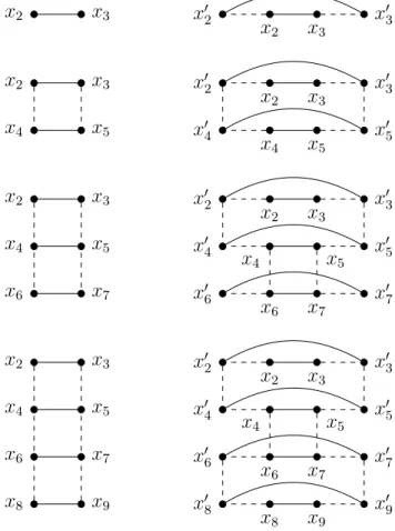
We will transform each weighted graph G on the vertices {x1, . . . , xk} to a weighted graphG′ on the vertices{w, x1, x2, . . . , xk, x′1, x′2, . . . , x′k}in such a way, that the matching M = {(x1, x′1),(x2, x′2), . . . ,(xk, x′k)} is a subgraph of G′, every edge of M gets weight 2 and the vertex wwill serve as the apex of G′.
We transform each component of G separately: A weighted ladder on h vertices is transformed into a weighted ladder of 2h vertices as follows. If (xi, xj) is an edge of weight 1 in G then in G′, both (xi, xj) and (x′i, x′j) are edges of weight 1. If (xi, xj) was an edge of weight 2 in G, then in G′ we alternately choose (xi, xj) or (x′i, x′j) to be an edge of weight 2 in G′ starting from the top of the ladder and doing differently ”above”
and ”below” each weight 1 edge, see Figure 7.
x2 x3
x2 x3
x′2 x′3
x2 x3
x4 x5
x2 x3
x4 x5
x′2 x′3
x′4 x′5
x2 x3
x4 x5
x6 x7
x2 x3
x4 x5
x′2 x′3
x′4 x′5
x6 x7
x′6 x′7
x2 x3
x4 x5
x6 x7
x8 x9
x2 x3
x4 x5
x′2 x′3
x′4 x′5
x6 x7
x8 x9
x′6 x′7
x′8 x′9
Figure 7. The transformation of the ladders.
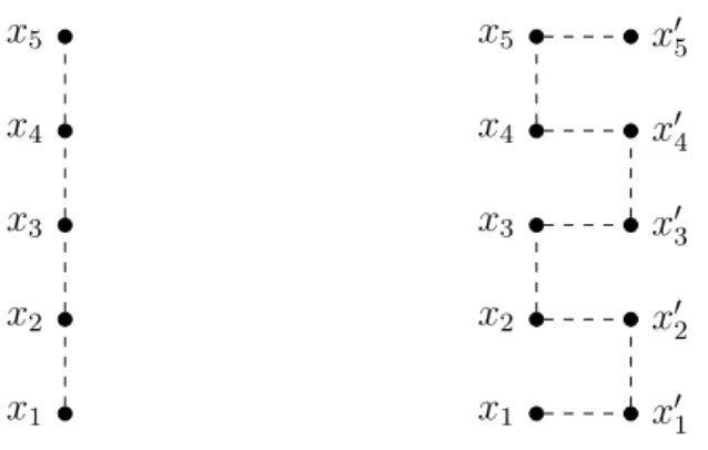
A path that consists of edges of weight 2 in (the residual part of) G is transformed as follows: If (xi, xj) was an edge of weight 2 in G, then in G′ either (xi, xj) or (x′i, x′j) is
9
an edge of weight 2 so that with the edges of M the resulting component of G′ is also a path, see Figure 8.
x1
x2
x3 x4
x5
x1
x2
x3 x4
x5
x′1 x′2 x′3 x′4 x′5
Figure 8. The transformation of the paths.
Note that this transformation doubles the number of vertices of the paths in the residual part, thus the difference in the number of their vertices is now four. To repair this we transform the apex ofGto a path containing two vertices connected by an edge of weight two and we attach this to the end of the shorter path restoring the length difference of the residual part to two. (Remember that we still have the apexw.) Thus this transformation produces properly laddered weighted graphs.
The transformed weighted graphs are compatible by the following argument. LetG1and G2be arbitrary weighted graphs from the H-maximal family andG′1, G′2their transformed counterparts from the MH-maximal family. Let (xi, xj) be (one of) the edge(s) that is contained in bothG1 and G2 but with different weight. Without loss of generality we can assume that it gets weight 1 in G1. We transformed G1 in such a way that G′1 contains both edges (xi, xj) and (x′i, x′j) with weight 1. However, since G2 contains the edge (xi, xj) with weight 2, we transformed it in such a way that in G′2 either the edge (xi, xj) or the edge (x′i, x′j) gets weight 2. This takes care of the induction step when k is odd.
If k is even: If k is even, then k −1 is odd, and there is an H-maximal family on k −1 vertices from which we can construct ⌊k−1k−21⌋
Hamiltonian paths. Unlike in the odd case, observe that this is just half the number of Hamiltonian paths we would like to construct, since if k is even then ⌊k−1k−21⌋
= 12 ⌊kk2⌋
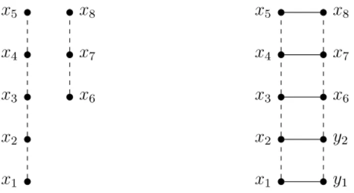
. We start with the exact same transformation of weighted graphs on the vertices {x1, . . . , xk−1} forming a H-maximal family to weighted graphs on the vertices {w, x1, . . . , xk−1, x′1, . . . , x′k−1}forming an MH- maximal family. We have two more vertices: xk and x′k that we did not use yet. Since k−1 is odd, the MH-maximal family on 2k−1 vertices consists of weighted graphs that have a non-empty residual part as every ladder contains an even number of edges from the prescribed matching of the MH-maximal family. Thus if we add the vertices xk, x′k connected by an edge of weight 2 to the shorter path in the residual part, we can complete the residual part of every weighted graph into a ladder, see Figure 9.
Thus for each weighted graph we increased the number of ladders by one. This by Lemma 2.5 doubles the number of Hamiltonian paths that the Z-swapping construction gives. Since for evenk we have 2 ⌊k−1k−21⌋
= ⌊kk2⌋
we are done. This finished the case when
k is even and the proof is complete.
10
x1
x2
x3
x4
x5
x6
x7
x8
x1
x2
x3
x4
x5
x6
x7
x8
y1
y2
Figure 9. With the two new vertices y1, y2, we can complete the residual part to a ladder.
Proof of Theorem1.4.We have already seen that it is enough to prove the statement when the number of vertices is odd. Then the statement of the theorem is equivalent to say thatH-maximal families exist on 2n+ 1 vertices for every n. Lemma 2.8 implies that this is true once we know the existence of MH-maximal families for all odd-element vertex sets of size at most 2n+ 1. Lemma 2.9 gives that this condition is always satisfied and
thus the proof of Theorem 1.4 is completed.
Remark. Consider the compatibility graph Gn of the Hamiltonian paths:V(Gn) is the set of Hamiltonian paths onnvertices and two such vertices are adjacent if the corresponding Hamiltonian paths are compatible. Theorem 1.4 determines the clique number ω(Gn) of this graph. Observe that the maximal clique is far from unique since in Lemma 2.5 we can use any ordering of the ladders. Thus we can construct 2l compatible Hamiltonian paths inl! ways there. By using Lemma 2.5 in the proof of Theorem 1.4, we can construct many cliques of maximal size in Gn. One can actually show that the number of maximal cliques in Gn is at least doubly exponential.
3. Hamiltonian-cycle-different paths
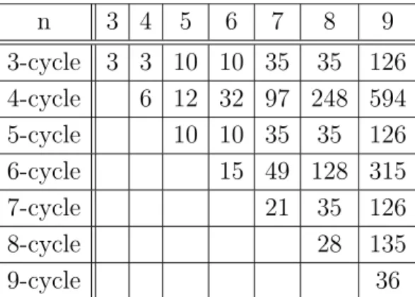
Now that we know the maximal number of triangle-different Hamiltonian paths, it is a natural question to ask what happens for other cycles. Observe that since odd cycles are not bipartite, the same upper bound holds forC2k+1-different Hamiltonian paths. For small ground sets Table 2 contains the largest families that we could construct using a computer.
Observe that in the case of odd cycles except at theC7-different paths on 7 vertices and the C9-different paths on 9 vertices, every value is best possible as they attain the upper bound (the number of balanced bipartitions). By the following Claim the two exceptional values are also best possible. We say that two Hamiltonian paths are Hamiltonian-cycle- different if their union contains a Hamiltonian cycle on their common vertex set.
Claim 3.1. The maximum number of pairwise Hamiltonian-cycle-different Hamiltonian paths on n vertices is at most n2
.
Proof. We use the trivial fact that a Hamiltonian graph does not contain a vertex of degree one. Let H be a family of Hamiltonian-cycle-different Hamiltonian paths. For every path in H we associate the two edges on their ends directed towards the center of the path. Observe that for distinct Hamiltonian paths in H we associated different edges, as their union does not contain a vertex of degree one. But there are exactly 2 n2
11
directed edges in the complete graph on n vertices and we associated two such edges to every path, thus 2|H| ≤2 n2
finishing the proof.
Remark. Note that for a fixedc, one can bound the number ofC(n−c)-different Hamiltonian paths on a ground set of size n in a similar fashion by a polynomial of degree c+ 2.
We present a construction that attains this bound when the size of the ground set is a prime number.
Claim 3.2. If p > 2 is a prime then there are p2
pairwise Hamiltonian-cycle-different Hamiltonian paths on p vertices.
Proof. Let us draw the ground set on the plane as a regular polygon. LetH consist of the Hamiltonian paths that do not contain two edges of different length. It is easy to see that
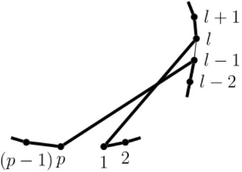
|H|= p(p−1)2 . If both H1, H2 ∈ H contain edges of length say l, then their union consists of every edge of length l, and this graph is a Hamiltonian cycle since the size of the ground set is prime. The Hamiltonian path {1,2, . . . , p} is compatible with every other path fromH that uses edges longer than one by the following argument. Let H2 ∈ H be a path that uses edges of length l. Since there is a single edge of length l that is missing fromH2, either both the edges ((p−l+ 1),1) and (p−l, p) are inH2 or both the edges (p, l−1) and (1, l) are in H2. In both cases we have a Hamiltonian cycle in the union, the latter case can be seen in Figure 10.
p 1 2 (p−1)
l−2 l−1
l l+ 1
Figure 10. The thick edges form a Hamiltonian cycle. We either have this or the symmetric situation when the two edges of lengthl are pointing towards the left side.
Two arbitrary Hamiltonian paths from H form a Hamiltonian cycle since we can straighten out one of them by relabelling the vertices so that it becomes the path {1,2, . . . , p}, while the other one will be transformed too, but it still connects vertices of the same difference modulo the size of the ground set thus the same reasoning applies.
4. Families of graphs with a triangle in every union
In the light of Theorem 1.3, one might find the following question natural. What is the maximal size of a family of n-vertex graphs with the property that every union contains a triangle? This is far easier than the intersection version. Let H, G be graphs. We say that H is a maximal G-free graph if it is G-free and adding any edge toH, the resulting graph has a (not necessarily induced) subgraph isomorphic to G.
Claim 4.1. Let G be a fixed graph. The maximal size of a family of graphs such that every pairwise union contains a copy of G is equal to the size of the family that consists of all the graphs that contain G as a subgraph and all the maximal G-free graphs.
12
Proof. The family that consist of all the graphs that contain G as a subgraph and all the maximalG-free graphs clearly has the property that every pairwise union contains a copy ofG. Now suppose that we have a family H of graphs with the property that every pairwise union contains a copy of G. Suppose that there is a graphH ∈ H that does not containG as a subgraph and that is not maximalG-free either. ThenH is a subgraph of a maximalG-free graphH′. Observe thatH′ ∈ H, since otherwise/ H∪H′ =H′ and there is no copy ofGin H′ a contradiction. Thus we can replace H with H′ without losing the property that in each union there is a copy of G. Thus one by one we can replace (push up) every graph inH that does not contain a copy of Gand is not maximal G-free to be
maximal G-free. This finishes the proof.
Proposition 4.1 is relevant to us when G is a triangle. Thus we see that when we do not add any restriction, the optimal families with the property that any union contains a triangle consist of the graphs that contain a triangle (the trivial ones) and the maximal triangle-free graphs. A less general superclass of the class of Hamiltonian paths is the class of trees. But determining the maximal size of triangle-different families of trees is also simple.
Claim 4.2. The maximum number of pairwise triangle-different trees on n vertices is 2n−1−1.
Proof. For the upper bound, observe that every tree is a bipartite graph. The number of (not necessarily balanced) bipartitions of [n] is 2n−1. We clearly cannot have two trees with the same bipartition, as the union would be bipartite. Moreover no tree corresponds to the bipartition of the ground set where one side is the empty set.
For the lower bound, we construct a large enough family of trees inductively. Forn= 2 the only tree on two vertices attains the upper bound. Suppose that we have a family Fn−1 of 2n−2 −1 triangle-different trees on the vertices {v1, . . . , vn−1}. We build a new set of trees Fn on the vertices {v1, . . . , vn} as follows. For each tree T ∈ Fn−1 let us fix two adjacent vertices x =x(T) and y = y(T) and we build two new trees Tx and Ty by connecting the new vertexvnas a leaf toxandy, respectively, without changing anything else in the tree. We also add the star centered at vn to Fn. Clearly every other tree is triangle-different from the star centered atvn. Two trees inFnthat are constructed from different trees in Fn−1 are triangle-different. And for a fixed T ∈ Fn−1, the union of the trees Tx and Ty contains the triangle x, y, vn. Thus Fn is a triangle-different family, with
size |Fn|= 2|Fn−1|+ 1 = 2n−1−1.
Remark. One can also ensure that the trees constructed in the proof of Claim 4.2 are either stars or double stars (two vertex disjoint stars and an edge connecting the center of the two stars) by the choice of the vertices x and y.
5. Open problems and concluding remarks
We conjecture that a relaxed version of Theorem 1.4 should be true for any odd cycle.
Conjecture 5.1. If k > 1 andn is large enough, the maximal number ofC2k+1-different Hamiltonian paths on n vertices is equal to the number of balanced bipartitions of the ground set n.
On the other hand the maximal number of C2k-different Hamiltonian paths is more than exponential (One can construct such a system of size nk
! using the simple method in Theorem 1 of [4]). An other significant difference between the even and the odd case is that the maximal number of even-cycle-different Hamiltonian paths is asymptotically
13
larger than the maximal number of C4-different Hamiltonian paths, as expected, see [4].
Thus one is tempted to think that we can observe the ”normal behaviour” for even cycles. For the following weaker version of Conjecture 5.1 we have additional supporting evidence.
Conjecture 5.2. Ifk >1then the maximal number ofC2k+1-different Hamiltonian paths on n vertices is at least 2n−o(n).
Generalizing the methods of present paper, we managed to show that Conjecture 5.2 is true when 2k is a power of two. But even in these cases our constructions are only asymptotically equal to the upper bound of balanced bipartitions. We consider this as the basis of a subsequent paper.
We also conjecture that the bound in Claim 3.1 can also be attained for composite integers.
Conjecture 5.3. The maximum number of pairwise Hamiltonian-cycle-different Hamil- tonian paths is n2
for every n.
The maximal number ofC4- orK4-different Hamiltonian paths is also an open question at the time, even the correct order of magnitude is unknown. For other open problems about the maximal number of Hamiltonian paths with some restrictions on the pairwise unions see: [1, 3, 4, 10–12]. Finally, in Table 2 we present the sizes of the largest families that we could construct for small ground sets and cycle lengths. This provides some experimental evidence for Conjecture 5.1 and Conjecture 5.3.
n 3 4 5 6 7 8 9
3-cycle 3 3 10 10 35 35 126 4-cycle 6 12 32 97 248 594
5-cycle 10 10 35 35 126
6-cycle 15 49 128 315
7-cycle 21 35 126
8-cycle 28 135
9-cycle 36
Table 2. Lower bounds to the maximal size of cycle-different Hamiltonian paths.
6. Acknowledgement
We would like to thank Kitti Varga and G´eza T´oth for the beautiful proofs of the com- binatorial identity in Lemma 2.8. We would also like to thank G´abor Simonyi, G´eza T´oth and J´anos K¨orner for their help which greatly improved the quality of this manuscript.
Finally we also thank many of our colleagues for encouragement and their interest in our progress.
References
[1] R. Aharoni and D. Solt´esz,Independent sets in the union of two Hamilotnian cycles, In preparation (2016).
[2] G. Brightwell, G. Cohen, E. Fachini, M. Fairthorne, J. K¨orner, G. Simonyi, and ´A. T´oth,Permutation capacities of families of oriented infinite paths, SIAM Journal on Discrete Mathematics24(2010), no. 2, 441-456.
14
[3] G. Cohen, E. Fachini, and J. K¨orner,Connector families of graphs, Graphs and Combinatorics 30 (2015), no. 6, 1417-1425.
[4] ,Path separation by short cycles, Journal of Graph Theory (2016), doi:10.1002/jgt.22050.
[5] D. Ellis, Y. Filmus, and E. Friedgut,Triangle-intersecting families of graphs, Journal of the European Mathematical Society14(2012), no. 3, 841–885.
[6] D. Ellis, E. Friedgut, and H. Pipel,Intersecting families of permutations, Journal of the American Mathematical Society24(2011), no. 3, 649–682.
[7] P. Frankl and M. Deza,On the maximum number of permutations with given maximal or minimal distance, Journal of Combinatorial Theory Series A22 (1977), no. 3, 352–360.
[8] J. K¨orner and C. Malvenuto, Pairwise colliding permutations and the capacity of infinite graphs, SIAM Journal on Discrete Mathematics20(2006), no. 1, 203–212.
[9] J. K¨orner, C. Malvenuto, and G. Simonyi,Graph-different permutations, SIAM Journal on Discrete Mathematics22(2008), no. 1, 489–499.
[10] J. K¨orner, S. Messuti, and G. Simonyi,Families of graph-different Hamilton paths, SIAM Journal on Discrete Mathematics26(2012), no. 1, 321–329.
[11] J. K¨orner and A. Monti,Families of locally separated Hamilton paths, arXiv:1411.3902 [math.CO]
(2015).
[12] J. K¨orner and I. Muzi, Degree-doubling graph families, SIAM Journal on Discrete Mathematics 27 (2013), no. 3, 1575–1583.
[13] J. K¨orner, G. Simonyi, and B. Sinaimeri, On the type of growth for graph-different permutations, Journal of Combinatorial Theory Ser. A116(2009), no. 2, 713-723.
Department of Control Engineering and Information Technology, Budapest Univer- sity of Technology and Economics
E-mail address, Istv´an Kov´acs:kovika91@gmail.com
Department of Computer Science and Information Theory, Budapest University of Technology and Economics
E-mail address, Daniel Solt´esz:solteszd@math.bme.hu
15