Economics of the welfare state
Economics of the welfare state
Sponsored by a Grant TÁMOP-4.1.2-08/2/A/KMR-2009-0041 Course Material Developed by Department of Economics,
Faculty of Social Sciences, Eötvös Loránd University Budapest (ELTE) Department of Economics, Eötvös Loránd University Budapest
Institute of Economics, Hungarian Academy of Sciences Balassi Kiadó, Budapest
Economics of the welfare state
Authors: Róbert Gál, Márton Medgyesi Supervised by: Róbert Gál
June 2011
ELTE Faculty of Social Sciences, Department of Economics
Economics of the welfare state
Week 1
Measuring social inequality
Róbert Gál, Márton Medgyesi
Topics
What is the subject of inequality measurement?
Inequality indices
• Basic indicators of dispersion
• Graphical representation of inequalities
• Basic indicators of dispersion
• Representation of inequalities by the Lorenz curve
• The Gini coefficient
• Axiomatic approach to inequality measurement
• Attributes of aggregate inequality indicators
• Generalized Entropy indices
• Decomposing inequalities
What is the subject of the measurement of inequality?
Basically we are interested in the distribution of material living standards (consumption-possibilities) among individuals.
Inequality of what?
The best basis of measuring consumption-possibilities could be wealth in the broad sense: everything that produces income in the present or the future:
• financial wealth: bank deposit, securities, etc.,
• material wealth: durable consumer goods, real estate, etc.,
• human capital: inherited abilities and learnt skills, knowledge
• entitlements to government transfers: e.g. to social security pension income.
All types of wealth result in a flow of income.
In what form?
Inequality of what?
YF = YM+YN
YF = total income
YM= monetary income: earnings, capital-income, financial transfers from the government
YN = non-monetary income: job satisfaction, leisure time, service of material wealth, value of self-produced consumption, non-financial transfers from the government YF the measure of individual consumption-possibilities
YF however is not a proper measure of individual well- being: e.g. it does not take into account uncertainty
In practice there are difficulties of measurement!
In case of non-monetary incomes: in almost every types.
In case of financial incomes, measurement of capital income (e.g. unrealized gain on securities) and the entrepreneurial income is difficult.
Inequality among individuals?
We measure income on household level even though we are interested in the distribution of living standards among individuals!
Solution: income per capita?
A
in separate household
B
in separate household
A and B together
Rent 30 30 50
Utilities 20 20 30
Food 15 15 30
Consumption goods 35 35 90
Total expenditure 100 100 200
Inequality among individuals?
Income per capita is NOT a proper measure
• Household public goods
• Distribution within the household: e.g. needs differ according to ages Equivalent income =total household income/number of consumption units in the household
OECD II scale:
• first adult: 1 consumption unit,
• further adults: 0.5 consumption units
• children (below 15) 0.3 consumption units
per capita income
OECD II.
scale
equivalent income
e=0,5 scale
equivalent income
One adult 1000 1,0 1000 1.00 1000
Two adults 1000 1,5 1333 1.41 1414
Three adults 1000 2,0 1500 1.73 1732
Two adults, 1 child < 5y 1000 1,8 1667 1.73 1732 Two adults, 2 children < 5y 1000 2,1 1905 2.00 2000 Two adults, 1 <5y, 1 15y 1000 2,6 1923 2.24 2236
Graphical representation of a distribution
Representation of information on
expenditure, consumption or income in
the form of diagrams is often very useful
in the analysis of inequalities.
Representations of basic indicators of dispersion
• Pen’s parade
• Frequency distribution
• Cumulative frequency distribution
• Lorenz curve
Height (income)
Rank of individuals poorest
richest
average
median
Representation of the distribution of incomes with the help of Pen’s Parade: ranking people by their income
Charting the income distribution
Source:
Tóth, 2005
Incomes
Rank of individuals
Flatter section: many people, small differences
Steep sections on the curve:
few people, large differences
Characteristics of dispersion
Charting the income distribution
Source:
Tóth, 2005
0 50000 100000 150000 200000 250000 300000 350000 400000 450000 500000 550000 600000 650000
1 18 35 52 69 86 10 3
12 0
13 7
15 4
17 1
18 8
20 5
22 2
23 9
25 6
27 3
29 0
30 7
32 4
34 1
35 8
37 5
39 2
40 9
42 6
44 3
46 0
47 7
49 4
51 1
52 8
54 5
56 2
income
Persons (ranked)
Pen’s parade in Hungary: income of people ranked by their per capita income in 1992
Charting the income distribution
Source: Tóth, 2005
Frequency distribution:
The diagram (histogram) illustrates the relative
frequency of individuals sorted into different
categories of expenditure.
For example the enclosed frequency distribution
shows that 20% of
individuals fall into the fourth category. [i.e.
f(4)=0.2].
0 5 10 15 20 25 30 35 40
1 2 3 4 5 6 7 8 9 10 11 12 13 14 15 Categories of expenditure
Percentage of population
Fre que ncy distribution f(y)
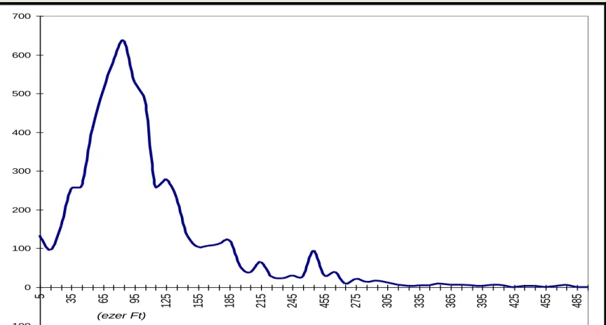
Charting the income distribution
Source: Tóth, mimeo.
-100 0 100 200 300 400 500 600 700
5 35 65 95 125 155 185 215 245 455 275 305 335 365 395 425 455 485
(ezer Ft)
Income distribution in 1992, illustration from the Hungarian Household Panel*
*Number of people in the HHP sample
Charting the income distribution
Source: Tóth, mimeo.
0 200 400 600 800 1000 1200
5 15 25 35 45 55 65 75 85 95 105 115 125 135 145 155 165 175 185 195 205 92
93 94 95 96 Number of persons
(1000)
Income (1000 Ft)
Income distribution in Hungary, 1992–1996*
*equivalent incomes deflated to 1992
Charting the income distribution
Source: Tóth, mimeo.
Cumulative frequency distribution: This graph
illustrates cumulative frequency – percentage of households on or below a given level of expense/income. Compared to the previous graph F(y) is the area below f(y) on the left side.
[F(4) = f(4)+f(3)+f(2)+f(1) = 20+35+12+4=71%]
0
10 20 30 40 50 60 70 80 90 100
1 2 3 4 5 6 7 8 9 10 11 12 13 14 15 Categories of expenditure
cumulative frequency (%)
Cumulativ e fre que ncy function F(y)
Charting the income distribution
Source: Tóth, mimeo.
Ratios of dispersion
Definition:
Ratios of dispersion measure the distance between two groups in the income distribution.
Typically the average income of the richest x%
of the population is divided by the average expenses/income of the poorest x%.
Different alternatives exist. Most frequently it is
based on the decile or the quintile of the
distribution (decile includes 10% of the total
population, quintile includes 20% of it).
Ratios of dispersion
The definition of a ratio of dispersion:
Based on group averages:
j group bottom
of income Average
i group top
of income Average
Based on cutpoints
(percentile ratio): Upper cutpoint for bottomgroup j i group for top
cutpoint Lower
Group i and group j can be defined as deciles (1/10), quintiles (1/5), quartiles (1/4), etc.
Incomes
Ranking of individuals
A few basic measures of income inequality
Lowest
decile 2nd decile
Highest decile
...
Note: high variation
on the margins, moderate
variation elsewhere Ratio of
the average of deciles
Percentile ratio
Ratios of dispersion
Source: Tóth, 2005
Ratios of dispersion
Advantages:
(+) The group-average ratios and percentile ratios are easy to interpret.
Disadvantages:
(–) The value of the group-average-ratio is highly sensitive to extreme incomes, particularly in case of small-sample estimations.
(–) No axiomatic basis, not derived from principles of equity.
Representation of inequalities by the Lorenz curve
Lorenz curve: The most common representation. The curve illustrates the
cumulative ratio of
expenditure on the vertical axis and the cumulative ratio of population on the horizontal axis. In this example 40% of the population possess less than 20% of the total
consumption expenditure.
0 10 20 30 40 50 60 70 80 90 100
0 20 40 60 80 100
Cumulative % of population
Cumulative % of consumption
Representation of inequalities by the Lorenz curve
If all individuals had the same income, i.e. the distribution of incomes was perfectly equal, the Lorenz curve would be identical to the diagonal (E: line of equality).
If one person had the total
income, the Lorenz curve would pass through points (0,0), (100, 0), and (100,100). This is the curve of „perfect inequality”.
Line (S): lower inequality Line (L): higher inequality What if they intersect?
E: Line of equality
L:Higher inequality S: Lower inequality
Cumulative decile shares (population)
Gini: surface between E and S divided by surface of the lower triangle Cumulative decile
shares (income)
Source: Tóth, 2005
Indices of aggregate inequality:
the Gini coefficient
The Gini coefficient is
related to the Lorenz curve representation.
The value of Gini equals the ratio of the area A and area A+B.
In the previous figure Gini equals 0 in the case of
perfect equality and 1 in the case of perfect inequality.
A
0 10 20 30 40 50 60 70 80 90 100
0 20 40 60 80 100
Cumulative % of population
Cumulative % of consumption
A
B
Indices of aggregate inequality:
the Gini coefficient
Definition:
The Gini coefficient is the most commonly used indicator of inequality.
The definition of Gini: ratio of the average absolute
income difference between every pair of the sample and the average income.
The Gini coefficient can range from 0 to 1. The value of 0 expresses total equality and the value of 1 maximal inequality. It measures the „deviation” from total
equality.
Formal definition:
Different formulae exist; the classical formula of Gini is :
Where yi and yj stand for individual income/consumption values, is the average, and n is the number of observations.
Indices of aggregate inequality:
the Gini coefficient
y n
n
y y
Gini
n
i
n
j
j i
) 1 (
2
1 1
y
Indices of aggregate inequality:
the Gini coefficient
Advantages (+) and disadvantages (–) :
(+) The coefficient is easy to understand because of its connection to the Lorenz curve.
(–) The coefficient is not additively separable: the Gini of the total population is not equal to the (weighted) sum of the Ginis of population subgroups.
Indices of aggregate inequality:
the Gini coefficient
The coefficient is sensitive to income-changes
irrespective of whether the change is taking
place at the top, the middle, or the bottom of
the distribution (all transfers of income
between two individuals have an effect
independently of their financial situation).
Axiomatic approach to the measurement of inequalities
In which distribution do you think inequality is higher?
1. A(5,8,10) B(10,16,20) 2. A(5,8,10) B(10,13,15)
3. A(5,8,10) B(5,5,8,8,10,10) 4. A(1,4,7,10,13) B(1,5,6,10,13) 5. A(4,8,9) vs B(5,6,10) ?
A’(4,7,7,8,9) vs B’(5,6,7,7,10) ?
See: Amiel és Cowell, 1999
Axiomatic approach to the measurement of inequalities
What kind of attributes should we expect of this kind of index?
1. Scale independence: if all incomes are multiplied by constant k, the inequality index should not change.
2. Population independence: if population increases in all income categories by the same ratio, the inequality index should not change.
Axiomatic approach to the measurement of inequalities
3. Symmetry: if two individuals transpose their income the value of the inequality index should not change.
4. Axiom of transfers (Pigou–Dalton): if income is redistributed from a richer individual to a poorer one (progressive transfer), so that their ranking does not change, the inequality index should decrease.
5. Decomposability: requirement of a coherent relationship between inequality in the total population and inequality in subgroups. If inequality in one subgroup increases (all
other things unchanged) total inequality should not decrease. Special type: additive separability.
Indices of aggregate inequality: the generalized entropy indices
Question: which axioms do or do not selected indices fulfill?
Theorem:
An index is consistent simultaneously with the axiom of scale
independence, population independence, axiom of transfers, and the axiom of additive decomposability if and only if it is member of the generalized entropy family of indices.
The formula of the Generalized Entropy Indices:
Where yi = income/consumption,
N = number of individuals, and is a parameter which weights the individuals of different levels of distribution.
N
i
i
y y GE N
1
2
1 1 1
) (
Indices of aggregate inequality:
the generalized entropy indices
2 1
1
2 1
1
1 1
) 2 2 (
log 1 .
) 1 (
1 log )
0 (
N
i
i N
i
i i
N
i i
y N y
y GE CV
y y y
y Theil N
GE
y y MLD N
GE
Depending on the value of parameter:
Indices of aggregate inequality:
the generalized entropy indices
Attributes of certain indicators
parameter index sensitivity
= 0 MLD middle incomes (mean log
deviation)
= 1 Theil index middle incomes
= 2 CV higher incomes (coefficient
of variation)
Indicators of aggregate inequality:
the standardized entropy indices
Advantages and disadvantages:
(+) Axiomatic basis: we know its attributes.
(+) GE(α) indices can be separated to ”subgroups” : the GE(α) index calculated on the total population is the
weighted average of the indices calculated on its
subgroups, where weights are the proportions of subgroups in the total population (this is not possible in the case of
Gini).
(–) Difficult to interpret (in contrast to Gini)
Decomposition of inequalities
• Inequalities are decomposed when one is curious about the extent to which inequalities among various social
groups, regions or income components are responsible for the total inequalities in a country.
• Inequalities can be separated to ”between group” and
”within group” components. The first one shows the
difference between the averages of people from different subgroups, and the second one shows the differences within the groups.
0 500000 1000000 1500000 2000000 2500000 3000000
25 50 75 100 125 150 175 200 225 250 275 300 325 350 375 400 401
ossz87 ossz01
1987
2001
Decomposition of inequalities:
distribution of income in total population, 1987 and 2001
Source: Tóth, 2005
200000 400000 600000 800000 1000000 1200000 1400000
Decomposition of inequalities: frequency distribution at different levels of education
0
25 50 75 100 125 150 175 200 225 250 275 300 325 350 375 400 401
0 200000 400000 600000 800000 1000000 1200000 1400000
25 50 75 100 125 150 175 200 225 250 275 300 325 350 375 400 401
1987 2001
primary
skilled worker
intermediate
higher education
Source: Tóth, 2005
Decomposition of inequalities
Decomposition of an additively separable index (MLD):
MLD= k vkMLDk + k vk log (1/k), Within group Between group
inequality inequality
Where vk =nk/n and k=k/