Selected Topics in the Theory of Concurrent Processes
Battyányi, Péter
Selected Topics in the Theory of Concurrent Processes
írta Battyányi, Péter Publication date 2015
Szerzői jog © 2015 Battyányi Péter
Tartalom
Selected Topics in the Theory of Concurrent Processes ... 1
1. Introduction ... 1
2. 1 Processes ... 1
2.1. 1.1 Definitions and notation ... 1
2.2. 1.2 The value-passing calculus ... 5
2.3. 1.3 Renaming ... 7
3. 2 Equivalence of processes ... 9
3.1. 2.1 Strong bisimulation and strong equivalence ... 9
3.2. 2.2 Observable bisimulation ... 13
3.3. 2.3 Equivalence checking, solving equations ... 16
4. 3 Hennessy -Milner logic ... 20
4.1. 3.1 Basic notions and definitions ... 20
4.2. 3.2 Connecting the structure of actions with modal properties ... 23
4.3. 3.3 Observable modal logic ... 25
4.4. 3.4 Necessity and divergence ... 27
5. 4 Alternative characterizations of process equivalences ... 27
5.1. 4.1 Game semantics ... 27
5.2. 4.2 Weak bisimulation properties ... 30
5.3. 4.3 Modal properties and equivalences ... 30
6. 5 Temporal logics for processes ... 32
6.1. 5.1 Temporal behaviour of processes ... 32
6.2. 5.2 Linear time logic ... 34
6.3. 5.3 Model checking in linear time logic ... 36
6.3.1. 5.3.1 Linear time properties ... 36
6.3.2. 5.3.2 Towards LTL model checking ... 39
6.3.3. 5.3.3 Büchi automata and model checking for LTL formulas ... 51
6.3.4. 5.3.4 Complexity of the LTL model checking process ... 54
6.3.5. 5.3.5 Fairness assumptions in LTL ... 54
7. 6 Computation Tree Logic ... 55
7.1. 6.1 Syntax of CTL ... 55
7.2. 6.2 Semantics of CTL ... 56
7.3. 6.3 Normal forms and expressiveness ... 59
7.4. 6.4 Relating CTL with LTL ... 60
7.5. 6.5 Model checking in CTL ... 61
7.5.1. 6.5.1 The crucial idea ... 61
7.5.2. 6.5.2 Searches based on the expansion laws ... 64
7.5.3. 6.5.3 Symbolic model checking ... 65
7.5.4. 6.5.4 Binary decision diagrams ... 68
7.6. 6.6 CTL* ... 73
7.6.1. 6.6.1 Basic notions and definitions ... 73
7.6.2. 6.6.2 Model checking in CTL* ... 74
8. 7 Hennessy -Milner logic with recursive equations ... 75
8.1. 7.1 Modal formulas with variables ... 75
8.2. 7.2 Syntax and semantics of Hennessy -Milner logic with recursion ... 77
8.3. 7.3 The correctness of CTL-satisfiability algorithms ... 79
8.4. 7.4 Equational systems with several recursive variables ... 81
8.5. 7.5 Largest and least fixpoints mixed ... 83
9. 8 The modal -calculus ... 84
9.1. 8.1 Logic and fixpoints ... 84
9.2. 8.2 Playing with modal -formulas ... 86
9.3. 8.3 Game characterization of satisfiability of modal -formulas ... 87
10. 9 Conclusions ... 91
10.1. 9.1 General overview of the approaches discussed ... 91
10.2. 9.2 Model checking in practice ... 92
11. 10 Appendix: The programming language Erlang ... 92
11.1. 10.1 Introduction ... 92
11.2. 10.2 Datatypes in Erlang ... 92
11.2.1. 10.2.1 Pattern matching ... 93
11.2.2. 10.2.2 Defining functions ... 94
11.2.3. 10.2.3 Conditional expressions ... 95
11.2.4. 10.2.4 Scope of variables ... 96
11.2.5. 10.2.5 The module system ... 97
11.3. 10.3 Programming with recursion ... 97
11.3.1. 10.3.1 Programming with lists ... 97
11.3.2. 10.3.2 Programming with tuples ... 102
11.3.3. 10.3.3 Records ... 103
11.4. 10.4 Concurrent processes ... 104
11.4.1. 10.4.1 Creating processes ... 104
11.4.2. 10.4.2 Simple examples ... 105
11.4.3. 10.4.3 Handling timeouts ... 108
11.4.4. 10.4.4 Registered processes ... 109
11.5. 10.5 Distributed programming ... 110
12. Hivatkozások ... 112
Selected Topics in the Theory of Concurrent Processes
1. Introduction
The aim of this course material is to give a little insight into the most widespread and fundamental techniques of the mathematical descriptions and modelling of reactive systems. The usual approach to sequential programs is to model the behaviour of a program as a sequence of actions which have the effect of changing the state of the program, the values assigned to the program variables, and at the point of termination the result, as the final state, emerges. So sequential programming is more or less a state transformation, from the input states it leads through a sequence of operations to a desirable final state. Unlike this approach a reactive or concurrent system can be viewed as a system sensitive to changes from stimuli or information from itself or from the environment.
In most of the cases, like operating systems, communication protocols, control programs, even termination is not desirable. These systems can be modelled as independent processes communicating with each other through some channels, but, in the meantime, doing their jobs independently. For a formal treatment several approaches were proposed, the most prominent ones among them were probably the theory of communicating sequential processes (CSP) of Hoare ([22]) and the calculus of communicating systems (CCS) of Milner ([32]). The two systems resemble in many aspects to each other. In this course material we have chosen Milner's approach.
The calculus of communicating systems offers an easy solution for modelling the participants of a communication process. Both the sender and the receiver are represented as a process, and the communication between them is taken place as a transition between the two processes, hence, the calculus chooses to model communication with message passing. In effect, the resulting system will be a labelled transition system, where communication is a synchronized communication. If value-passing is added to the original model, we also have a structure modelling communication with shared variables.
The course material focuses both on the definitions and the key notions in the field of CCS and on the various results concerning the semantical aspects of labelled transition systems. The first chapter defines processes as constituents of labelled transition systems, it gives the structural operational semantics of the transitions and then even presents the notion of the value passing calculus. The next chapter is about process equivalences: it is a nontrivial question whether two processes have the same meaning, how to interpret the equivalence of processes at all. If one process is a specification and the other one is an implementation: how do we know that the implementation meets the requirements of the specification? Then Hennessy -Milner logic as a basic tool for process behaviour is introduced. In the fourth chapter another approach of process equivalence is discussed: we present the results of Stirling ([37]) on characterizing process equivalence by two player games. The next two chapters treat the model-theoretic aspects of the behaviour of transition systems in detail. Timed logics are introduced, which enable us to pose questions relating temporal behaviour of processes. These questions are sought to answer as questions of formula satisfiability, in our present terminology, as questions of model checking: given a labelled transition system and a formula, is it the case that the transition system, or some of its states satisfy the given formula? The last but one chapter is about processes defined by recursive equations (cf.
[30]). Finally, the last chapter introduces the modal -calculus together with a game semantic tool for model checking (see [37]).
The author would like to thank the reviewer, István Majzik, for his thoroughness and for the invaluable comments and suggestions he contributed with to this course material.
2. 1 Processes
2.1. 1.1 Definitions and notation
We define the notions of sequential and concurrent processes, which are the underlying notions of the calculus of communicating systems introduced by Milner in his works [32] and [33]. Processes themselves can be considered as states of a complex system and actions that are the transitions from one state to another. This
gives rise to various approaches of describing the behaviour of these systems. One of them is the theory of labelled transition systems, along which we will elaborate the theory of concurrent processes in this course material. First of all, following [32] we are going to give the definiton of a labelled transition system.
1. Definition Assume we have a set called the set of actions and a set called the set of states. A labelled transition system (LTS) over is the pair with for every . If , then we call the source, the target and we say that is a derivative of under . In notation: . If
, where , then if . In case of
we simply put . 2. Remark
1. If the set of actions is not important, we may simply write for the LTS in question. With the above
notation .
2. Another usual terminology for labelled transition systems is as follows. Assume we have a set for the set of actions and a set for the set of states. A labelled transition system (LTS) over is a pair , where . We prefer the former definition of an LTS, however.
3. In the literature a labelled transition system is sometimes termed as an abstract reduction system ([26]).
Throughout this course material we stick to the term of labelled transition system.
We are going to define the labelled transition system of concurrent processes as a special kind of LTS. First we define a restricted process language, where is the set of process names and is an index set. We denote the elements of either by upper case letters, or, when, later on, we accept the temporal logical approach to LTSs, by lower case letters: usually , will stand for processes. Let be given as a set of names.
Assume , and . Then is the set of actions, where the
elements of are called observable (or external) actions and is called an unobservable (or internal) action.
The processes are considered with name parameters, e.g, will indicate that are the parameters of . Assume furthermore that is a function such that and
. Then is called a renaming function, and the result of the application of to the expression will be denoted by . Then our first process language can be defined by the grammar
where , , and is a Boolean expression. The elements of , , , are called process expressions. The intuitive meaning of the various constructs is as follows: the sum can be considered as a sort of nondeterministic choice. The sum can have an action iff any of its summands has that action. Parallel composition acts very similar to sum, with the exception that it may trigger a synchronization between its two sides when an action and its co-action is executed by the two components. In this case a silent action takes place, concerning the whole system. Finally, restriction serves as means for hiding actions of processes, thus constraining them to exert their effect within the LTS given. Process expressions can thus be process names, sums of process expressions, parallel composition of process expressions and expressions obtained by previously defined ones by restriction, renaming or the if-then-else construct. When the index set is finite,
say , then we write instead of . We assume that the
unary connective renaming is the strongest one, then is stronger than summation and composition.
Composition is stronger than the parenthesis of the if-then-else construct. Moreover, and are associative to the left. We omit parenthesis if possible, though, for the sake of readability, we write instead of
.
A process expression is a process if, for the process names of , there is a set of defining equations , where the process names in each are either belong to or are processes themselves.
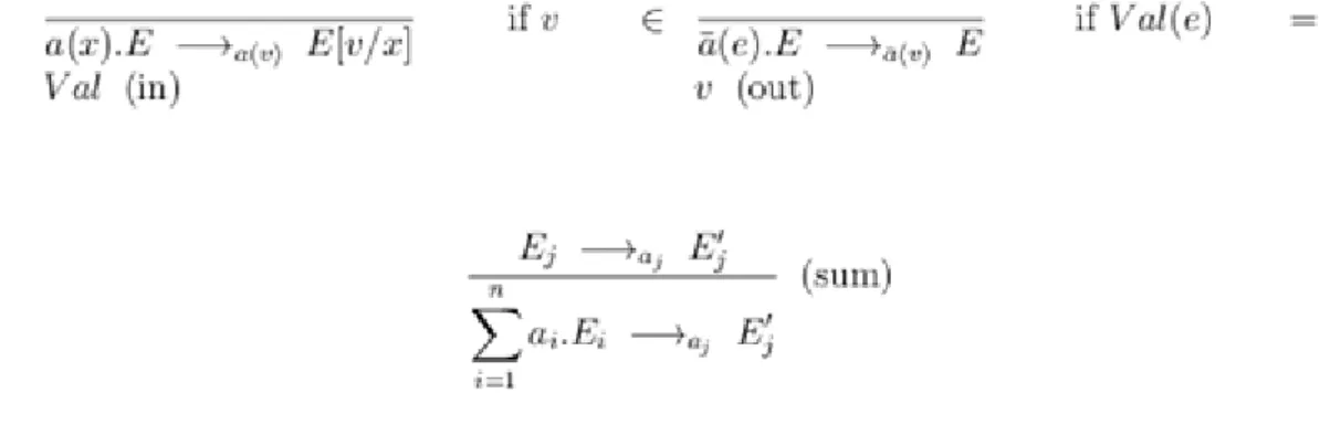
Next, we define the transition relations for this restricted process language. We give the transitions in the form of derivation rules, which means that if the upper relations are derivable then we can conclude the derivability of the lower ones. The rules for summation have no premises, this means they constitute the axioms in the calculus.
Figure 1 captures the axioms and derivation rules of the emerging calculus.
We illustrate by some examples how to define processes and interpret their actions. Drawing labelled graphs may help with understanding the behaviour of processes. The vertices of the behaviour graphs are process expressions, the vertices are connected with an edge labelled by an action if there is a transition between the two process expressions with action . Each transition derivable of a vertex is indicated in the behaviour graph.
3. Example[37]
Then can be considered as a clock which ticks perpetually. The only action can do is , this can be seen by the trivial derivation below.
4. Example[37]
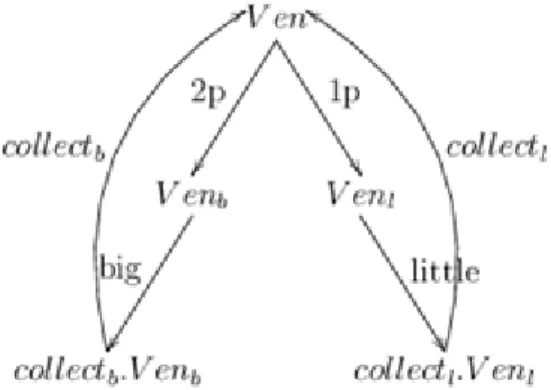
The above example defines a vending machine . The machine can accept two coins, a 2p and a 1p coin. By applying the binary choice operator this means that the machine either continues with the process expression , which means that after the button is depressed and a big item is collected the machine reverts to its starting point , or it continues with , and in this case depression of the button and collecting a small item returns the process to the point .
This can be depicted by the behaviour graph of Figure 2. All transitions of the graph can be justified with the proof rules as above. For example:
5. Example[37] Our next example is a buffer with capacity two illustrated in Figure 3. Its process identifiers are numbered according to the possible combination of bits it can contain. In total, the buffer has six process names, namely for each . Let (and ) represent the input (and output) of some value . Then the defining equations are as follows.
6. Example[32] A slightly modified version of the buffer of capacity when, instead of choosing different process names, we assume that can take as arguments arbitrary finite sequences of length at most . In this case the definition of the buffer takes the following form.
where denotes the empty sequence and is the concatenation of and the one-element sequence . 7. Example[32] We intend to define a process so that its execution should behave as a scheduler for the tasks
and . We require the scheduler to meet the following specifications:
1. should occur cyclically, beginning with , 2. and should occur in this order for every .
For the time being we give the scheduler as a sequential process, later on we are going to define it as a network of concurrent processes. The process names have two parameters: when writing we mean by this that it is to come next and, given , we know that has already been executed while
waits for their turn to come next.
and is understood as .
8. Example[32] Our final example in this row describes a counter. Unlike the processes defined so far, the counter has infinitely many states.
Observe that indicates when the value encoded in the process decreases to 0 again.
2.2. 1.2 The value-passing calculus
For the sake of a more compact treatment we modify our calculus a little. We assume that not only the process identifiers, or agent names, can have parameters, but also the action names can take arguments. Our modified syntax is as follows: we assume that a fixed set of values is given, and every process name has an arity, which is the number of arguments it can take. The actions can have one or zero argument. Assume that the possibly indexed symbol denotes an expression built from variables taking values from , value constants and arbitrary function symbols. Moreover, let denote Boolean expressions and assume is a set of process variables. Let , where is the set of process names of some arity. Then the process expressions is the set defined by the following grammar:
We assume the following precedence order is valid for our operators: renaming is the strongest of all connectives, which is followed in decreasing binding power by restriction and prefixing, then parallel composition, summation and the if-then-else construct. This means e.g. that by we
understand .
In the expression all occurrences of are treated as bound. Prefixing with co-names, that is the expressions , does not create new bindings. As before a process is a set of equations of the form , with and , where the process names in every are a subset of
and contains no free variables except for .
The proof rules for prefixing and summation must be modified accordingly. The new rules are indicated in Figure 4, where denotes the result of substituting the value in place of the variable .
Let us demonstrate in a few examples the expressive power of our process language. Our first examples are copier machines, the first one simply takes an input and discards it at once, the second one takes as argument a number and a text , and outputs as a result copies of .
9. Example[37]
takes a value in and immediately outputs it. The size of the transition graph of depends on the number of elements in . The multiple copier asks for a number and a text, which is copied times.
Figure 5 gives us some insight into the operation of .
The next example makes use of the if-then-else construct to define a process that sieves odd and even numbers.
10. Example[37]
If is even, then the output of is , else it is . For example, let
Then for we have
The next example shows interactions between the copier machine and a new process . writes a file which can serve as an input for .
11. Example[37]
The machine is the same as in example 9. Then we may have the following transition sequence:
. In the example above the justification of each transitional step is straightforward, let us pick out one of them.
Though the full calculus allows a more concise notation for processes, everything that can be expressed in the full calculus can be described in the restricted calculus as well. We are not going to give the translation, we demonstrate only in some examples how the translation is accomplished. Let us consider Example 11. Assume is some value-set. Then the variable in can take either value in , which is reflected in the translation by defining a new action for every . Similarly, to every , we assign a new action name .
In this manner we can give the restricted equivalents of the processes of the full calculus.
2.3. 1.3 Renaming
We should recall from Section 1.1 that renaming is a function such that it obeys some special properties. Namely, and . As an illustration of the usefulness of renaming we redefine the scheduler of Example 7, this time building it from smaller concurrent components (cf.
[37]). The scheduler is an organiser of tasks, symbolizing the beginning and the end of the -th task.
The tasks begin with the first one and continue operating one after the other but a new operation cannot begin until the previous operation has not finished. Thus must come in this order, and each must be followed by a before a new appears in the sequence. We choose the seemingly obvious solution first.
Let be a cycler, defined as . As a first attempt we build the required scheduler as a ring of cyclers, where action is used for task initiation, action for termination, and actions and for synchronization. Let
To achieve a more compact form in our notation we denote the reflexive and transitive closure of our transition
relation by . Thus iff or there is a such that and .
We indicate by superscript the sequence of transitions leading from to if it is also interesting.
Thus and . We take and internalize
them by . That is, we form . Intuitively, by
internalizing with the states has the following effect. Each cycler is an independent process in itself, which means it is capable of performing actions indicated in its process equations, that is, they can perform even the actions or , where is understood as . But, since these actions were reserved for synchronizing purposes, it is desirable that none of them should appear as activities of the processes observable from outside. This means that these transitions can only take place in the course of a synchronization, in the form of an unobservable transition . For instance, the four-element scheduler
is illustrated in Figure 6.
There is a delicate bug, however, in the behaviour of . Namely, since synchronizes between and in a way that happens before , and happens after , this means that cannot have its turn before the synchronization takes place, especially could only happen after . To remedy this problem Milner ([32]) introduces the following solution: should be
and the renaming is as above. Then we obtain the -task scheduler as .
3. 2 Equivalence of processes
Process expressions are intended to describe states of complex systems. It is natural to ask when two systems can be inferred to be the same by checking their states and transition relations. Checking the defining equations of processes alone is not enough for distinguishing two processes, for example, giving different names to the process identifiers of a process does not change its behaviour. We are going to distinguish coarser and finer notions of equivalence depending on whether we contemplate a process from the inside or from an outside position as an external viewer. In this sense we talk about strong and weak equivalence of processes.
3.1. 2.1 Strong bisimulation and strong equivalence
First of all, we define the strong equivalence of processes. Our intention with the definition is to obtain a notion of interchangeability of processes in a sense that equivalent processes could be interchanged in process expressions without changing the meanings of the processes deduced in some way from their induced labelled transition systems. It is an interesting question in itself, how we are going to understand the meaning of a process as a transition system. Our main approach will be to treat processes equal with respect to their behaviour if a bisimulation relation, in the sense to be defined, can be set up between them. As an example, take the two processes
We have the feeling that the two processes are the same though their implementations differ. By looking at the transition diagrams of the processes in Figure we can convince ourselves in this.
12. DefinitionLet be a process. Then a trace of is a finite or infinite sequence of actions
such that . We write for the set of all traces of .
Obviously, a process can have many traces.
13. Example[37] Consider the following three vending machines (Figure 7):
The set of traces of the processes are the same. Consider a new process, however,
where denotes here, and in what follows, the process which does nothing. So a drops two coins into the machine, then chooses to drink a tea, and, having had their tea, expresses satisfaction by a visible gesture.
We say that a trace is completed if no more moves are possible finishing that trace. Let
. Then, for the process we have
which is the single completed trace of the process. On the other hand has a completed trace
A similar statement holds for , too.
Consider now the operator which replicates the successor of a processs, that is
It is straightforward to check that the set of completed traces of and are different.
14. Definition A binary relation on processes is called a bisimulation if for every and
1. if , then there is an with and ,
2. if , then there is an with and .
If a bisimulation between the two processes and exists, then we say that and are strongly bisimilar with respect to . We indicate this by .
15. Definition Let us define the relation
If , we call the processes and strongly bisimilar.
16. Example Let
Then is a bisimulation, thus and are strongly bisimilar. No other relations among hold, as it can be seen easily.
17. Example As expected, the vending machines in Example 13 are not strongly bisimilar. Let us check the pair
, for example. Assume is a relation such that and
. Then either and
or and
. But none of the pairs of processes obtained can be
bisimilar. Consider e.g. . Then
and . The other cases are treated similarly.
18. Example[37] Consider the processes
and
Let be the following family of processes
where and . Then
is a bisimulation for the pair .
We are going to state and prove a theorem describing the relation between strong bisimulations with respect to a relation and the relation .
19. TheoremLet be a labelled transition system. Then is an equivalence relation, and it is the largest bisimulation over . Moreover, iff, for each action ,
• when , then there exists such that and and
• when , then there exists such that and .
Bizonyítás.Let be a labelled transition system.
• First of all, we prove that is an equivalence.
1. : the identity relation is a bisimulation that contains .
2. implies : if , then there is a bisimulation for which
. Then the relation is a bisimulation proving , too.
3. and implies : in this case and
for some bisimulations and . Then is a bisimulation containing , where .
• Since
every bisimulation is contained in . We have to show that is a bisimulation. By the symmetry of , it
suffices to prove that and imply and for some state .
Assume and . Then there is a bisimulation such that . But, by definition, there exists such that and . The latter implies , as required.
• The 'only if' part follows from the fact that is a bisimulation. Assume therefore that, for each , (1) and (2) of the theorem hold for and . Consider the relation
It can be proved readily that is a bisimulation containing . [QED]
20. DefinitionA process context is a process expression containing a whole. Formally,
21. DefinitionLet be a relation over . Then is a congruence with respect to the operations of the process language, if it is an equivalence relation and, for every and every context , it follows
that .
22. Definition Let be a relation over . Then is a process congruence if is an equivalence, and
if , then
Every congruence is a process congruence, but we will see an example of a process congruence which is not a congruence. The following lemma shows that strong bisimulation is a congruence with respect to the operations of our process language. The straightforward proof of the lemma is omitted.
23. Lemma Let . Assume is a process, is a set of actions, is an action and is any renaming function. Then
1.
2.
3.
4.
5.
6.
7.
24. Example In the previous chapter we defined a buffer of capacity two, let us now define a buffer of capacity .
We claim that this is strongly bisimilar to the process consisting of the parallel composition of buffers of capacity 1. That is,
Hint: take
such that . is a bisimulation containing .
3.2. 2.2 Observable bisimulation
Hitherto we were concerned ourselves with a strict notion of equivalence of processes, taking into account all the transitions a process can make. But from the point of view of an external observer the internal actions of a process can be of no importance or unknown. Thus, we intend to develop a theory reflecting equivalence in the case when only external actions are observed.
25. Definition Let denote , that is, can be obtained from by a finite sequence of zero or more transitions. Furthermore, let be the observable action preceded and followed by an arbitrary finite number of silent transitions, that is, .
Sometimes it is convenient to explicitly indicate the silent activity involved in the sequence of transitions . For this reason we introduce the notation:
If and are sequences of actions we write , or simply , for their concatenation.
In a way analogue to that of the previous section, one can define bisimilarity of processes based on observable transitions. It is termed as weak bisimilarity. The intuition behind is to grasp when two processes seem to be identical from the perspective of an outer observer.
26. Definition A relation between processes is a weak bisimulation provided that whenever and
1. if , then there is an such that
2. if , then there is an such that
and are weakly bisimilar with respect to if there is a weak bisimulation such that . In notation: . The following proposition gives an equivalent characterization of weak bisimulation, the proof of which is straightforward.
27. Proposition The relation is a weak bisimulation iff whenever and
1. if , then there is an such that
2. if , then there is an such that
28. Example[32] Consider the following two processes drawn in Figure 8.
The relation is a weak bisimulation between the two
processes. However, there can be no strong bisimulation containing . The reason is that choosing we had to find such that , which is impossible.
29. Example[32] Let
Then is a weak bisimulation. Observe, e.g., that for we
can choose .
Let
30. Proposition implies .
31. Proposition is an equivalence relation and it is the largest weak bisimulation.
Bizonyítás.Analogous to that of Theorem 19. [QED]
32. Remark It is easy to check that for any process we have . First, if , that is
, then with . Conversely,
means with . If , the result is obvious. Otherwise, and
. On the other hand, observe that . If a bisimulation relation contained , then it would have to contain as well, but they are obviously not bisimilar.
The previous remark involves that weak bisimulation, as defined here, is not a congruence relation with respect to the process forming operations but it is still a process congruence, as we will see below. However, with a slight modification we can obtain a relation from which is also a congruence. Though in the rest of chapter we use Definition 26 for weak congruence, since its definition is a little simpler, and being a process congruence, it is most of the time enough for our purposes. In the definition below denotes the congruent subset of , and is the original weak bisimilarity of Definition 26.
33. Definition iff
1. , and
2. if , then there is an such that for some and , and
3. if , then there is an such that for some and
This implies that if and are initially unable to perform a silent action, then follows from . It can be shown that is the largest subset of which is a congruence with respect to the process language operators.
As we mentioned previously, weak equivalence is also a process congruence.
34. Lemma Let . Assume is a process, is a set of actions, is an action and is any renaming function. Then
1.
2.
3.
4.
5.
6.
3.3. 2.3 Equivalence checking, solving equations
A possibility for proving equivalences of processes is to set up an equational theory and to argue by equational reasoning. It is inevitable that our theory be defined so that process equivalence is a congruence, and establishing equivalence in this way makes it possible to deduce strong or weak equivalence in the sense of the previous sections. For this purpose, the observational congruence proved to be a good candidate. We list the equations used most frequently in the equational arguments.
35. Lemma Let the variables and stand for process expressions. Then
The expansion law transforms parallel composition of sums into a sum of parallel compositions. Let , then
where and
The expansion law can be simply justified by the rules of parallel composition and sum.
Let be any expression. A variable is sequential in if it does not occur within the scope of a parallel composition in . is guarded in if it is within the scope of an expression , where . For example, in is both guarded and sequential. In is guarded, but not sequential.
36. Theorem[32] Assume the expressions contain at most the variables free . Let these variables be sequential and guarded in . Then the set of equations has a unique solution .
By this we have two more rules, the so-called recursion rules.
• If , then .
• If and is guarded and sequential in , and if and is guarded and sequential in ,
and , then .
37. Example Let us check that the following processes defined by the equations below are equal.
Then, since equality is a congruence with respect to the process operators, applying the relations of Lemma 35 we have the following equations:
On the other hand
Both and are guarded and sequential in the equations obtained, thus Theorem 36 on the unicity of recursive equations can be applied. In this case, if we use the notation , then it turns out
that and , hence, obviously, , and
Theorem 36 gives the result.
The following example checks whether an implementation fulfills the requirements of a specification. The processes were conceived based on an idea in [1].
38. Example Let
the process is meant to represent a computer science department, where the only action visible from outside is the action of writing publications. First of all, for the safe operation of a computer scientist a coffee
machine is needed, which fact is well-known due to Pál Erdő. The coffee machine does nothing but supplies us with coffee, provided a coin is inserted beforehand. The
describes its operation. The individual computer scientist should be
that is, a computer scientist publishes documents, inserts a coin into the coffee machine, and wishes to drink either a coffee or a tea. For the sake of simplicity, let us assume for the moment that our department consists of one computer scientist only. Our aim is to prove by equational reasoning that
where . Applying the equations listed in Lemma 35 and the expansion law several times we obtain the following sequence of equations:
where . Since is guarded and sequential in , by
Theorem 36, we can conclude that . The situation is similar when we have different computer scientists , , defined by the analogy of . It is left to the reader to prove that in this case the equation
is valid, too. In other words, if is the specification of a process, and
is an implementation, then the implementation meets the requirements of the specification. Observe that the structure of is the same as that of in Example 13, only the names of the actions differ.
As a more complex example, let us generalize the buffer of Example 24 to a buffer of capacity storing now an arbitrary sequence of values with length . Let be fixed, assume and ranges over . Then
If is empty, we simply write . Let , . We connect cells in the usual way: the outgoing port of one cell is the incoming port of the another. Thus
Let . We can use the more intuitive notation
. In what follows, let . We claim
39. Theorem .
First of all, we prove 40. Lemma
Bizonyítás. By the expansion law,
Taking into account that, by the remark following Definition 33, it holds that and , we obtain the result. [QED]
By the previous lemma it is enough to suppose that the linked cells are of the form
. We denote this by , where . By
Theorem 36 it is enough to prove that satisfies the same equations as . 41. Lemma
Bizonyítás. The proof goes by induction on . The case is simply the definition of . Assume we have the result for , let us prove
By the expansion law we have , which is
by Lemma 40. Next, we show
If :
Let :
Finally, let such that
By this the proof is complete. [QED]
4. 3 Hennessy -Milner logic
4.1. 3.1 Basic notions and definitions
In this chapter we widen our examination concerning processes. We are going to describe the behaviour of processes with the help of a modal logic, the so-called Hennessy -Milner logic. The formulas of the logic are built from the logical constants and , propositional connectives and the modal operators ("box ") and ("diamond ") for any set of actions . The inductive rule for building formulas is as follows.
42. Definition
1. The propositional atoms and are formulas.
2. If and are formulas, then and are also formulas.
3. If is a formula, is any set of actions, then and are formulas.
Let be the modal logic obtained in the above definition. We stipulate that the modal operators bind stronger than the propositional connectives, thus the outermost connective of is conjunction.
Furthermore, instead of (and , resp.) we write (and
, respectively).
We can define the meaning of formulas in connection with processes. When a process has the property , we say that realises, or satisfies . In notation: . The realisability relation is defined by induction on the structure of formulas. Below, and denote processes, is a set of actions.
43. Definition 1.
2.
3. iff and
4. iff or
5. iff for every and such that
6. iff for some and such that
For example, expresses the ability to carry out an action in , while denotes the inability to perform an action in .
44. Example Consider the clock of Example 3. Then, for example, .
By definition,
45. Example[37] Consider the vending machine in Chapter 1. We demonstrate that, for example, , that is, after inserting two pence, the little button cannot be but the big one can be depressed.
46. Notation Let be the set of all actions, that is, , where is the set of observable actions.
In the modal prefixes we use the notation for and for . E.g., a process realizes iff for every if , then . Especially, expresses a deadlock, or termination, of . Or expresses the fact that the next action of must be .
With the notation above one can express certain properties of necessity or inevitability. For example, for the vending machine of Example 4 we have . That is, after the insertion of a coin, the machine does not stop, and its next action is that the button big can be depressed. Or,
, that is, the third action must be a collecting of either a little or a big item.
We can express negation in a natural way in our logic. For every formula we define its complement . 47. Definition
1.
2.
3.
4.
5.
6.
For example, .
48. Proposition iff .
Bizonyítás.The proof goes by induction on the structure of . [QED]
Observe, that . Although in the presence of negation or complementation many logical connectives or modal operators become superfluous in the sense that they are expressible from the existing ones, making use of them often facilitates the tasks of building formulas in a language. In this spirit, we may introduce implication in the modal language as well, with its well-known meaning. Thus,
or, in the presence of negation,
In the sequel, we feel free to use implication, as well.
Actions in the modality prefixes may contain values, as well. For example, the copying machine
of Example 9 has the property , which
means that after accepting the value the machine is only capable of outputting the same value . After setting a domain we could augment our satisfaction relation with the clauses for quantifiers:
49. Definition
1. iff
2. iff
We obtain a logic of the same expressibility but without quantifiers, if we introduce infinitary modal logic. The sets of formulas are:
50. Definition
1. The propositional atoms and are formulas.
2. If and are formulas, then and are also formulas, where is an arbitrary finite or infinite index set.
3. If is a formula, is any set of actions, then and are formulas.
The semantics is modified accordingly:
51. Definition
1. iff, for every ,
2. iff there is an such that
Moreover, and can be seen as abbreviations for and , respectively. Let us denote the logic obtained by . Now we can express quantified formulas in as infinite conjunctions or
disjunctions. For instance, is interpreted as
.
4.2. 3.2 Connecting the structure of actions with modal properties
Processes also have an inner structure, which can enable us to draw conclusions on modal properties of processes without directly appealing to the realizability definition again and again. The following lemma highlights some typical cases of this sort.
52. LemmaLet , denote processes, be a process name and be a set of actions.
1. If , then and .
2. If , then iff .
3. If , then iff .
4. iff for all .
5. iff for some .
6. If and , then .
Bizonyítás.We give the details for some of the cases.
• (1.) iff , but implies
and . But , so the first statement is vacuously true. By the same reasoning, since
, .
• (4.) By definition of the sum, iff for some . By this, the statement follows.
[QED]
53. Example Now we can show some properties of transition systems without having direct recourse to the
definition of transitions. For example, let us prove , that is,
after a coin is inserted and an item is chosen, an item can be collected.
Next, our intention is to define an operation on modal formulas such that it captures the effect of restriction on actions. Our purpose is that iff should hold. In what follows, let for any set of actions .
54. Definition 1.
2.
3.
4.
5.
6.
With the definition as above, the next lemma states the main property of the operation .
55. Lemma iff .
Bizonyítás.By induction on . We pick only one case, namely, the case of .
• Assume and . Then there is an and such
that . By the induction hypothesis, . But , hence , this
is in contradiction with .
• Assume and . Assume and . Then
and . By inductive hypothesis, , and since and were arbitrary, this contradicts the assumption .
[QED]
4.3. 3.3 Observable modal logic
Formerly, we distinguished observable and silent actions of processes. Since modal properties are closely connected to transitions of processes, it is natural to ask, how to express properties in relation to observable or silent activity only. An appealing approach to define modalities in connection only to silent activities is restricting the set of processes reachable in one step to processes reachable by a sequence of silent steps.
56. Definition
1. iff for all , if , then
2. iff there exists such that and
where indicates zero or more silent steps. A process has property , if, after implementing any amount of silent activities, it has property . Likewise, for fulfilling a process must be able to evolve, through some silent activities, to a process which fulfills . Interestingly, neither , nor can be expressed in our modal logic . We are going to prove this fact.
To this end, we note that two formulas and are equivalent, if, for every process , iff . Thus, is not definable in if there is a such that is not equivalent to any formula of . We find that is such a formula for any . Let us consider the following two sets of processes for every
.
Then for every , while , since a sequence of silent actions starting from can end up with an . On the other hand, for each formula there is a such that iff , which is a consequence of the next proposition. By this, we obtain that no formula can express the statement . In what follows, let denote the complexity of the modal formula , that is, the number of logical connectives and modal operators in the formula.
57. Proposition Let be a formula of , assume . Then, for every , iff .
Bizonyítás.For the statement is trivial. Assume we know the result for , let and . We give the details only for the case of . If , then, by Lemma 52, we have
and . If , then, again by Lemma 52, iff and
iff . Now the induction hypothesis applies. [QED]
We may define the new modalities
We have
Similarly,
If stands for observable actions, then
For example, means that a process is unable to carry out an observable action, an example can be . A process is stable, if it cannot execute an unobservable action, hence satisfying the formula . expresses that a process is stable, and every observable action coming next is not an element of
. is called an observable failure for if .
58. Example Let us consider the vending machines and of Figure 7.
Assume the set of actions is . We claim that and have the same observable failures. Since both processes and the processes derived from them are stable, we only have to look for such that , where . We can read from Figure 7 the possible transition
sequences starting from or from . For example,
and
. For every , it can be shown by induction on that is an observable failure for iff it is an observable failure for .
By introducing the new modalities as primitives, we obtain a new modal logic, the observable modal logic , of which the formulas we define below.
59. Definition
As before, negation can be expressed by defining the complement of a formula.
4.4. 3.4 Necessity and divergence
Assume we intend to express the property that the next observable action will be a . If we try , the formula fails to express it, as the following process shows
can act forever in silent mode, but . In fact, in we are not able to express the intended property. Instead, we introduce new notation to be able to indicate that a process is going to operate forever or not. We say that diverges, if there is an infinite sequence . The notation indicates that diverges, and indicates that converges. Let
Let us demonstrate now that divergence is not expressible in observable modal logic.
60. Proposition Let . Then and the process 0 are equivalent in , that is, for every ,
iff .
Bizonyítás.By induction on . It is enough to restrict ourselves to the modal operators. More closely, it is sufficient to consider , since and can be handled by Lemma 52. Likewise for . But, trivially, iff and iff , hence the induction hypothesis applies. [QED]
But, on the one hand, , which is obviously false for 0. If we augment with the newly defined modalities, we obtain the observable modal logic with divergence . Now we can express that is the
next observable action by the formula .
5. 4 Alternative characterizations of process equivalences
5.1. 4.1 Game semantics
In Chapter 2 we had a closer look at process equivalences. Since the behaviour of processes can be depicted by their transitions, it is a natural demand to ask whether two processes defined by different descriptions denote actually the same process if they are compared by their sets of transitions. These comparisons can be made interactive if we consider solving process equivalence as a game where at each step observers can freely pick a
transition of one process, and then try to match it with a transition of the other process. We follow the account of Stirling ([37]) in the course of this chapter.
Assume we have processes and , and two players (refuter) and (verifier). An equivalence game for processes and is a sequence , , ..., of processes, where , and the th element is defined in the following way:
• Player chooses an , then has to choose an .
• Player chooses an , then has to choose an .
We indicate by the fact that there is a game-sequence , , ...,
with . The game continues until both players can take their steps. Player wins if the game stops with 's turn. Otherwise, if the game stops with 's turn or is infinite, then it is a -win. More
formally, is an -win iff there is such that either , and there
does not exist for which or the other way round. With the notation of modal logic:
and or and . All the other situations are considered - wins.
61. Example Let and , consider . Then, if the refuter
always chooses the part of , we obtain a -win. However, choosing the part of by the refuter, we obtain an -win immediately, since, if the refuter chooses from the pair , this cannot be answered by the verifier.
We describe informally what we mean by a strategy for and . A strategy for is a prescription: given a state of the game it settles what state or to choose, where or for some . Likewise, given a state ( , respectively) and an action ( , respectively), a strategy for gives such that (gives such that , respectively). Since the prescriptions for and use only previous states of the game, we call them history-free strategies. We say that a game is won by (by , respectively), if (resp. ) has a winning strategy for the game. We say that two processes and are game equivalent if the game is won by the verifier.
62. Example A winning strategy for in the game is "at always choose ",
where .
63. Example Let be defined as usual, and let . This game is an -game. If the refuter follows the strategy "at choose ", then he wins the game. For the next move of the verifier can only be , and at the state , the game finishes with the refuter's move
: the refuter wins.
Before we state and prove the next theorem we have to say some words about ordinals. Ordinal numbers can be viewed as the order types of well-ordered sets starting from the natural numbers. They can be imagined as the results of an infinite sequence of constructions: take for zero, then for 1, for 2, etc. In general, will be the next ordinal, while a limit ordinal is the union of all smaller ordinals . In what follows, the processes are all countable, so definitions by transfinite recursion make use of countable ordinals only.
64. Theorem Let be a game. Then either or has a history-free winning strategy.
Bizonyítás. Let be a game, assume , when is defined inductively as
, when , and , when and . Then the set of
possible positions for is
We define a set inductively, characterizing those states of the game from which an -win position can be
reached. Let be the set of immediate -wins and let
for . Then
Let . It is obvious that Force is the set of positions from which can win the game. This means, if , then the game is won by , otherwise it is won by . [QED]
We mention that game equivalence is an equivalence relation between processes. Though the previous proof is not constructive, it is applicable in case of finite processes.
65. Example Let
We claim that and are not game equivalent. To this end, it is enough to give a winning strategy for . The winning strategy is depicted in Figure , where ellipses represent the states of the game from which an - move, and rectangular forms represent the states from which a -move follow. In Figure abbreviates
and stands for . The state of the game
represents a winning position for the refuter, since the refuter's previous move was and from it is impossible to perform a -transition.
66. ExerciseDraw the game graph for , where
In Chapter 2 we talked about process equivalences. It should not be a surprise that game equivalence and process equivalence coincide.
67. Lemma Two processes , are game equivalent iff they are strong bisimulation equivalent.
This means that checking game equivalence is an algorithm for verifying bisimulation equivalence, too.
5.2. 4.2 Weak bisimulation properties
Defining game makes sense for observable actions, as well. The difference from the previous notion is that this time we ignore silent actions when matching transitions. Let , be two processes. An observable game
is a sequence of pairs , , ..., , such that , and the
th element is defined in the following way: if and
• player chooses an , then has to choose an ,
• player chooses an , then has to choose an .
We indicate by the fact that there is a game-sequence , , ...,
with .
The game is an -win, if can perform an action , where , such that cannot answer this step. Every other situation is considered a -win. Since can always take the step , we may assume that a game is either finite, in which case it is an -win, or infinite, and then it is a -win.
68. Exercise Show that the game is won by the verifier, where , and are
defined as in Example 66 with the exception that .
We also have the coincidence of weak bisimulation equivalence and observable games.
69. Lemma Processes and are observable game equivalents iff they are weak bisimulation equivalents.
70. Exercise([37]) Let , where
Show that , where , by presenting an observable equivalent game
for the pair .
5.3. 4.3 Modal properties and equivalences
Another possibility to define equivalence of processes is relating them through their model properties.
71. Definition Let be formulas in . We say that the properties of are shared by (in notation:
), if, for every , implies . and share the same properties iff
and . In notation: .
In what follows we are going to consider only modal equivalence, that is the property . Special cases are when is the empty set or is the set of all modal formulas of . If is the empty set, then, for any and
, . On the other hand, for , we have the following theorem of Hennessy and Milner.
72. Theorem If , then , where is the set of formulas of .
Bizonyítás.By induction on the structure of . We consider only the case . Assume and
. Let with . Then there exists with . implies
, and applying the induction hypothesis we obtain , as desired. Hence . [QED]
The converse of the theorem is not true, it does hold, however, for a narrower set of processes. A process is immediately image finite if, for any , the set is finite. is image finite, if every descendant of , that is, the processes in the set are immediately image finite.
73. Theorem If and are image finite and , then . Bizonyítás.Define the relation
We prove that is a bisimulation, from which the statement of the theorem follows. Let , assume
and . Since and , we can conclude that the set
is non-empty. By image finiteness of , . Since , we
have , such that and . Then, with , and
, contradicting the hypothesis . [QED]
Image finiteness is necessary in the previous theorem, as the following example shows.
74. ExampleLet and let be
Let be and be . Then , since, obviously, . On the other
hand, we are going to prove in Proposition 80 that, for every , iff . This
implies .
We mention that in the case of , defined in Section 3.1, we obtain a necessary and sufficient characterization of bisimulation equivalence.
75. Theorem iff .
We remark that the notions above translate fairly smoothly into the case of observable logic, as well. If we define games as above, with the exception that every transition is exchanged by its observable counterpart , we can state theorems similar to the above ones. In these theorems game equivalence is corresponding to observable game equivalence, and strong bisimilarity is corresponding to (weak) bisimilarity.
76. TheoremTwo processes and are observable game equivalents iff .
77. Proposition If , then .
The analogue of Theorem 73 is also true with a corresponding notion of observable image finiteness. is immediately observably image finite, if, for every , is finite. is observably image finite if, for every , is immediately observably image finite.
78. Proposition If and are observably image finite and , then .
The importance of the Hennessy-Milner theorems lies in the fact that they provide criteria, for a wide set of processes, to decide weak or strong bisimilarity.
79. Example Consider the two processes and , where
We can conclude, by Theorem 72, that , if we take into account the fact that and .
6. 5 Temporal logics for processes
6.1. 5.1 Temporal behaviour of processes
The logic considered so far is capable of describing properties of processes referring to a point in time which is in a bounded distance from the present. For example, if we define
inductively and , we can see that and , or
but and so on. In general: processes are able to make a certain amount of ticks but none of them is capable of infinite ticking as is. Moreover, we are not able to express this property of in the logic defined so far, as the following reasoning shows. Assume there exists expressing the property of ticking forever. Then we must have and . But the following assertion contradicts this hypothesis.
80. Proposition Let such that . Then there exists such that , if .
Bizonyítás. We consider only the case . Assume . By Lemma 52, and
. Then, by the induction hypothesis, there exists such that for every . We may assume . Since in this case , for every , choosing we have
whenever . [QED]
Temporal properties of processes are described by their runs rather than by their individual transitions. A run of a process is a sequence of subsequent transitions either infinite or stalled, which means it is impossible to take a transition from the last element of a finite run. It turns out that bisimulation preserves runs in the following sense.
81. Proposition Let . Then
1. if , then there are such that
,
2. likewise, if , then there are such that
.
It turns out that bisimilar processes behave in the same way concerning their runs. We can introduce notation for expressing temporal behaviour. A set of useful and sufficiently general notations could be the following. First of all, we can quantify the set of runs: prefixing a modal formula with an should mean for all runs, and prefixing a formula with an should read as there exists a run. Moreover, for formulas and let
satisfy iff there exists such that and for every we have . With this in hand if we define the formulas of a logic with negation as
we obtain a variant of the logic defined by Clarke et al. (). Observe that, since contains negation, the operators and connectives previously present in and missing from can be expressed in . For example, . We can define the semantics of the new operators by considering runs:
Observe that the fact that a run is a completed sequence of transitions was important in the definition here:
as defined here would not be the same without this supposition. In order to avoid such inconveniences, in the sequel we are going to assume that every state has a possible next state. We will make this stipulation in due time. With these new operators many interesting properties can be expressed for runs:
Then
where , and reads as eventually , moreover, and reads as always . Observe that
In particular and .
Despite the fact that is more expressive than our previous modal logic, it is still unable to express certain properties, like the property of perpetual ticking. A remedy for this situation can be to provide the logic with temporal operators relativized to sets of actions like , where a run should satisfy iff every transition
of it is in , and each process of the run satisfies . In this case expresses the ability of perpetual ticking. In what follows, we pay a short visit to the temporal logics most common in the literature, and investigate in more detail the solutions offered for their model checking problems.
6.2. 5.2 Linear time logic
In the remainder of this chapter we give a short account, following the monographs of Baier et al., and that of Huth and Ryan (cf. [6], [24]), of the temporal logics most extensively used. The simplest one of them is probably the logic of linear time (LTL), which, despite its relative simplicity, is capable of expressing many valuable properties of processes, as we are going to see that in some examples soon. (In fact, we define PLTL, that is, propositional linear time logic.) Linear time temporal logic models temporality along one possible thread of time. Following the conventions in the literature we introduce LTL with negation and with variables for atomic propositions. Let denote the set of atomic propositions, let , , , . We assume that always contains and . We suppose that holds, and is false in every state. Then the syntax of propositional LTL is given in Backus -Naur form as follows:
82. Definition
The operator is termed as the next state and as the until operator. We define our transition system in a more general context. We assume that, in addition to , some more atomic propositions can hold in our states.
First, we define a Kripke structure over a given set of atoms .
83. Definition Let be a set of atoms, be a set of states and is a binary relation. If , then is a Kripke structure over . Throughout this chapter we assume that is a finite set of states.
Let be a sequence of states such that . Then is a path starting form
. We apply the notation for the segment of starting with . We interpret the truth value of a formula of LTL in a Kripke structure as follows.
84. Definition Let , be a Kripke structure and be a path.
Then is satisfied in with respect to (in notation: ), if one of the following cases holds:
• and ,
• and and ,
• and it is not the case that ,
• and there is a such that and for every we have ,
• and .
We omit from , if it is clear from the context.
It is not hard to obtain the interpretations of the temporal operators in case of a labelled transition system. The
role of here is played by the set , hence paths are of the forms ,
where , or simply if we do not want to indicate explicitly the actions performed.
Traditionally, several other connectives are defined in LTL. We list some of them, though, in the presence of negation, all the operators introduced can be expressed by the temporal operators and . We can consider e.g. the unary operators and known as for some future state, and for all future states, resp., or the binary
operators and called as release and weak until. Let us give the Kripke-style semantics of the new operators:
85. DefinitionLet be a Kripke-structure and be a path. Then
• iff there is an such that
• iff, for every ,
• iff either there is an with and, for all ,
or, for every ,
• iff either there is an with and, for all ,
or, for every ,
We write , if all execution paths starting from satisfy . We say that and are equivalents (in notation: ), iff for every and in we have iff . Without proof we list some useful equivalences. If we put them together we can even infer of the adequateness of the set . The first set of relations show that and , and and are duals of each other, is dual to itself. We assume that the unary connectives bind most tightly, then the binary temporal connectives are stronger than the binary logical ones.
86. Example
The above equations testify that many connectives of LTL are expressible by each other. The following can be said about the expressiveness of the connectives of LTL. The next operator is orthogonal to each of the connectives, that is, cannot be expressed, nor can be used in expressing the other ones. Moreover, the sets
, , each form an adequate set of connectives, where . The
operator is called the release operator and has a remarkable property as follows.
87. Definition A formula is in release positive normal form (RPNF) if it is of the form defined by the Backus - Naur notation below:
where is atomic.
That is, a formula in release positive normal form can contain negations only in front of atomic statements. The following assertion holds true.
88. LemmaFor every LTL formula there is a in RPNF such that .
Bizonyítás. The statement follows by successively applying for the equivalences above together with the
relation . [QED]
This means, if we adopt the operator as primitive in our language of LTL, it is no more a restriction to suppose that every formula is in RPNF. The transformation yields a formula not considerably longer than the original one.
6.3. 5.3 Model checking in linear time logic
6.3.1. 5.3.1 Linear time properties
As in the previous section, we will follow the state-based approach. This means that we consider relations that refer to the state labels, i.e., the atomic propositions that hold in the states. Action labels are not emphasized, though we may indicate them as the labels of the transitions. In this section we assume that all transition systems are transition systems without final states. We add arrows pointing to trapping states to final states of transition systems. That is, we augment our LTS, if necessary, with states having only outgoing transitions pointing back to the states in question. Then we create edges from all final states to one of the trapping states, thus obtaining an infinite path in the graph from that previously final state. In this and the next chapter, we prefer the notation etc. for the states than the capital letter notation we used in the previous chapters. We may alter the two notations, at the same time keeping in mind that a process description and a state of a transition system are not the same.
89. DefinitionLet be a transition system, where is the set of states, and are the sets of actions and atomic statements, respectively, and is the (possibly empty) set of initial states. If is a path, then
is the trace of path . Moreover, and
. If is the finite initial segments of , then .
We remark that the notion of trace defined here differs a bit from the one defined when we considered LTS in relation with its transitions. As we mentioned earlier, especially in the model checking problems, LTS also have an underlying Kripke structure, and in some cases more emphasis is laid on the Kripke structure aspects of an LTS. The notion of trace defined above lays emphasis on the atomic statements true in the subsequent states of a sequence of transitions. We indicate explicitly in what sense we are talking about traces, if it should not be clear from the context.
90. DefinitionA linear time (LT) property is a subset of . A transition system has LT-property
(in notation ), if . A state has LT-property ( ) if
.
Trace equivalence can be characterised by equivalence with respect to linear time properties, as the following lemma states.
91. Lemma Let TS and TS' be transition systems without terminal states and with the same set of propositions AP. Then the following statements are equivalent:
1.