Optimization of hadoop cluster for analyzing large-scale sequence data in
bioinformatics
Ádám Tóth, Ramin Karimi
Faculty of Informatics University of Debrecen adamtoth102@gmail.com
raminkm2000@yahoo.ca Submitted: June 13, 2017 Accepted: January 23, 2019 Published online: February 27, 2019
Abstract
Unexpected growth of high-throughput sequencing platforms in recent years impacted virtually all areas of modern biology. However, the ability to produce data continues to outpace the ability to analyze them. Therefore, continuous efforts are also needed to improve bioinformatics applications for a better use of these research opportunities. Due to the complexity and diver- sity of metagenomics data, it has been a major challenging field of bioinfor- matics. Sequence-based identification methods such as using DNA signature (unique k-mer) are the most recent popular methods of real-time analysis of raw sequencing data. DNA signature discovery is compute-intensive and time-consuming.
Hadoop, the application of parallel and distributed computing is one of the popular applications for the analysis of large scale data in bioinformatics.
Optimization of the time-consumption and computational resource usages such as CPU consumption and memory usage are the main goals of this paper, along with the management of the Hadoop cluster nodes.
Keywords: hadoop, optimization, next-Generation Sequencing, DNA signa- ture, resource management
doi: 10.33039/ami.2019.01.002 http://ami.uni-eszterhazy.hu
187
1. Introduction
Since the announcement of the human genome project completion in 2003 [8], Next- Generation Sequencing (NGS) technologies have revolutionized exploration of the secrets in the life science. Due to extraordinary progress in this field, massively parallel sequencing of the microbial genomes in the complex communities has led the advent of metagenomics techniques.
Metagenomics, a high-throughput culture-independent technique has provided the ability to investigate the entire community of microorganisms of an environment with analyzing their genetic content obtained directly from their natural residence [9, 15].
Along with technical advances of sequencing, mining the enormous and ever- growing amount of data generated by sequencing technologies is now one of the fastest growing fields of big data science, but there are still a lot of difficulties and challenges ahead. Real-time identification of microorganisms from raw read sequencing data is one of the key problems of current metagenomics and next- generation sequencing analysis. It has a pivotal role for pathogenic diagnostics assays to consider an early treatment.
Sequence-based identification of the species can be classified into two groups:
Assembly and alignment-based approaches and alignment-free approaches [7].
Due to the difficulties, technical challenges, and computational complexity of alignment and assembly-based approaches, they are not applicable for complex sequencing data such as metagenomics data. Moreover, they are expensive and time-consuming.
Reads generated by high-throughput sequencing technology are short in length and large in volume, very noisy and partial, with too many missing parts [9, 19].
They contain sequencing errors caused by the sequencer machines. Another chal- lenge is repetitive elements in the DNA sequence of species. As an example, about half of the human genome is covered by repeats [16]. These challenges cause inca- pability and unreliability of the results in alignment-based identification. Thus, it is necessary to develop efficient alignment-free methods for phylogenetic analysis and rapid identification of species in Metagenomics and clinical diagnostics assays, based on the sequence reads. Several alignment-free methods have been proposed in the literature to address this problem. One of the latest methods is using DNA signature that plays the role of fingerprints for microbial species.
DNA signature is a unique short fragment (k-mer) of DNA, which is specific for a species that is selected from a target genome database. DNA signature can be obtained for every individual species in the genome databases by screening and counting the frequency of k-mers through the entire database. The term k- mer refers to the existence of all the possible substrings of length k in a genome sequence. Each k-mer that appears once in a genome database is a unique DNA signature for the related sequence containing that k-mer. Since comparing k-mers frequencies are computationally easier than sequence alignment, the method can also be used as a first stage analysis before an alignment [10].
Considering the large size of genome databases, searching the unique DNA signatures (k-mers) needs powerful computational resources and it is still time- consuming. This problem can be solved by incorporating parallel and distributed computing.
Several tools and algorithms of k-mers frequency counting and DNA signature discovery have been proposed in the literature. Some of them use the applications of parallel and distributed computing. Hadoop and MapReduce are among these applications. The Apache Hadoop software [18], is a platform for parallel and distributed computing of large data set and MapReduce [3] is a programming model for parallel and distributed data processing.
In this paper, we have proposed optimization techniques to reduce time-consum- ing and to use less computational resources. Accordingly, we designed the nodes and managed the performance of the nodes in the Hadoop cluster. Managing the CPU consumption and memory usage according to the size of data and the number of maps, monitoring and comparing the running time of the maps were other issues that we have considered in this study.
The aim of this research is to enhance the possibility of using ordinary computers as a distributed system, in order to allow the process of searching DNA signatures and k-mers frequency to be applicable for the entire research community.
2. Background
This section contains a brief overview of the basic concepts that are used in this paper.
2.1. Next-Generation Sequencing (NGS)
Next-generation sequencing (NGS) refers to methods that have emerged in the last decade. NGS technologies allow simultaneous determination of nucleotide se- quences of a variety of different DNA strands. It provides reading of billions of nucleotides per day. NGS is also known as massive parallel sequencing. The NGS has dramatically improved in recent years, making the number of bases that can be sequenced per unit price has grown exponentially. Therefore the new platforms are distinguished by their ability to sequence millions of DNA fragments parallel to a much cheaper price per base. In this technology, experimental advances in chemistry, engineering, molecular biology and nanotechnology are integrated with high-performance computing to increase the speed at which data is obtained. Its potential has allowed the development of new applications and biological diagnos- tic assays that will revolutionize, in the near future, the diagnosis of genetic and pathogenic diseases [1, 12–14, 17, 20].
2.2. Metagenomics
For the first time, the word “metagenomics” appeared in 1998 in the article written by Jo Handelsman [6]. Metagenomics is the study of the entire genetic material of microorganisms obtained directly from the environment. The main goals of metagenomics are to determine the taxonomic (phylogenetic) and functional com- position of microbial communities and understanding that how they interact with each other in the term of metabolism. Historically, the bacterial composition was determined by culturing bacterial cells, but the majority of bacteria are simply not cultivated. You can isolate a separate species and study its genome, but this is long, since there are many species together as a diverse community [5, 19].
2.3. Alignment-based analysis
One of the most effective and convenient methods for classification and identi- fication of sequence similarity is an alignment method. Alignment of the new sequences with already well-studied makes it possible to quantify the level of simi- larity of these sequences, as well as to indicate the most likely regions of similarity structures. The most commonly used programs for the comparison of sequences are BLAST, FASTA and the Smith-Waterman (SW) is the most sensitive and popular algorithm is used. The applications of sequence alignment are limited to apply for closely related sequences, but when the sequences are divergent, the results cannot be reliable. Alignment-based approaches are computationally complex, expensive, and time-consuming and therefore aligning large-scale sequence data is another limitation [11]. Inability of this method becomes more visible when facing massive sequencing reads in metagenomics.
2.4. Alignment-free analysis
Alignment-free methods are an alternative to overcome various difficulties of tra- ditional sequence alignment approaches, they are increasingly used in NGS se- quence analysis, such as searching sequence similarity, clustering, classification of sequences, and more recently in phylogeny reconstruction and taxonomic assign- ments [2, 4]. They are much faster than alignment-based methods. The recent most common alignment-free methods are based on k-mer/word frequency. DNA signature is a unique short fragment (k-mer) of DNA, which is specific for a species that is selected from a target genome database. DNA signature can be obtained for every individual species in the genome databases by screening and counting the frequency of k-mers through the entire database [10].
3. System model
In our investigation we create a cluster which consists of three computers (N1, N2, N3). The next table (see Table 1) shows the main components of them.
Node Processor Memory Hard disk
N1 Intel Core i3-2120 (3.3 GHz) 4 GB ST1500DL003-9VT16L (1.5 TB) N2 Intel Core i7-3770K (3.5 GHz) 16 GB WDC WD20EZRX-00DC0B0 (2 TB) N3 Intel Core i7-4771 (3.5 GHz) 16 GB TOSHIBA DT01ACA200 (2 TB)
Table 1: Main components of the nodes
To run Hadoop, Java is required to be installed and we use version of 1.8.0- 111. Throughout the investigation on each computer runs Ubuntu 14.04.5 Server (64-bit) and to collect information of utilization of cpu, memory, I/O of the nodes we choose collectl tool which is suitable for benchmarking, monitoring a system’s general heath, providing lightweight collection of device performance information.
In this paper the input data is part of the genome database which contains k-mers.
In our case k is 18, so that each file contains lines of 18 character lengths. We configure block size as the input for running the maps to be exactly 1GB so after loading the data into HDFS it will be divided into 1GB parts. We considered 1GB of RAM to each map process. We downloaded the bacterial genome database in FASTA format from the National Center for Biotechnology Information (NCBI) database. The size of this database is 9.7 GB after decompression. In order to generate k-mers from the FASTA files, we used GkmerG software to generate all the possibilities of 18-mers from individual bacterial genomes of the whole database with a total size of 177.35 GB. The result is a file containing a single column of k-mers with length 18. The length of k-mers can differ according to the needs.
Since, the aim of this paper is optimizing the process of searching the frequency of k-mers, the large file must be split in the same size (1GB) for each map to compare the running time of the maps, therefore we assume that the large file is pre-sorted and the same k-mers is not located in different files after splitting. For the real data processing we have to split the large file in an intelligence manner.
During our investigation we use one of the example program on the input data called grep that extracts matching strings from text files and counts how many time they occurred.
Hadoop is designed to scale up from single servers to thousands of machines, each proposing local computation and storage, giving the opportunity to the system to be highly-available. Usually in practice the chosen machine, which is the master node, does not store any data so it does not do the job of datanode. In our case there is only one “real” datanode (N3) which is opposite of Hadoop’s principles.
However, in our scenario in that way we can focus on the efficiency of the utilization of resources during running Hadoop and also with that configuration we decrease network traffic as low as possible. Because YARN only supports CPU and memory reservation with our setting we can discover the crucial point of the system. The nodes of the cluster are configured in the following way: N1 is the master node (Resourcemanager runs on it), on every occasion only the applicationmaster (AM) runs on N2 because 15 GB RAM is given to AM and on N3 the default setting remains (1536MB) and Hadoop chooses N2 to start running AM. 14GB is given to yarn on N3 meaning that maximum 14 maps can run simultaneously. Every block
is located physically on N3 and every container (so every map process) runs on N3 except the AM.
The following table (see Table 2) includes the main features ofCases.
Case Number of map Size of the block Size of dataset Given memory to N3
a 1 1 GB 1 GB 14 GB
b 2 1 GB 2 GB 14 GB
c 3 1 GB 3 GB 14 GB
d 4 1 GB 4 GB 14 GB
e 5 1 GB 5 GB 14 GB
f 6 1 GB 6 GB 14 GB
g 7 1 GB 7 GB 14 GB
h 8 1 GB 8 GB 14 GB
i 9 1 GB 9 GB 14 GB
j 10 1 GB 10 GB 14 GB
k 11 1 GB 11 GB 14 GB
l 12 1 GB 12 GB 14 GB
m 13 1 GB 13 GB 14 GB
n 14 1 GB 14 GB 14 GB
Table 2: Scenario A
4. Numerical results
4.1. Scenario A
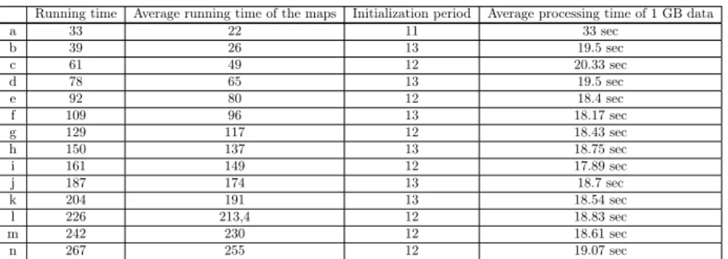
As it is indicated earlier we use collectl to get information about the utilization of resources of the nodes. It works under linux operating system and basically reads data from /proc and writes its results into a file or on the terminal. It is capable of monitoring any of a broad set of subsystems which currently include buddyinfo, cpu, disk, inodes, infiniband, lustre, memory, network, nfs, processes, quadrics, slabs, sockets and tcp. Collectl output can also be saved in a rolling set of logs for later playback or displayed interactively in a variety of formats. The command can be run with lots of arguments and it can be freely customized in which mode collectl runs or how its output is saved. Below (see Table 3) we can see some results about running times. The first column indicates the whole running time of the application, the second one shows the mean running time of the map jobs, the third one the initialization period which means after hadoop starts some time is needed before launching map jobs (e.g. deciding which node will be the master node). The last column represents the whole running time divided by the number of map jobs.
It can be seen that as more map processes are running in parallel the average processing time of 1 GB data starts to decrease then it remains around a constant value.
Running time Average running time of the maps Initialization period Average processing time of 1 GB data
a 33 22 11 33 sec
b 39 26 13 19.5 sec
c 61 49 12 20.33 sec
d 78 65 13 19.5 sec
e 92 80 12 18.4 sec
f 109 96 13 18.17 sec
g 129 117 12 18.43 sec
h 150 137 13 18.75 sec
i 161 149 12 17.89 sec
j 187 174 13 18.7 sec
k 204 191 13 18.54 sec
l 226 213,4 12 18.83 sec
m 242 230 12 18.61 sec
n 267 255 12 19.07 sec
Table 3: Results in connection with running times
4.1.1. Results in connection with the node where AM is located
As mentioned earlier the AM runs on this node on every occasion. Because of the rounding and the way of configuring collectl figures might not demonstrate the exact beginning of the running process but the deviation is very little. Because of the lots of data the graphs would be unclear so the achieved results are divided into two groups according to the number of processed blocks:
∙ Number of processed blocks are odd (1,3,5,7,9,11,13)
∙ Number of processed blocks are even (2,4,6,8,10,12,14)
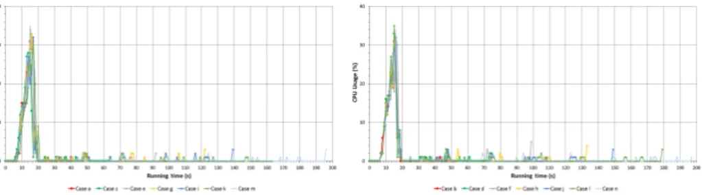
Figure 1: CPU usage of N2
On Figure 1 the data of cpu usage of N2 node is shown. As on N2 just the AM runs it can be seen after the jobs are initiated CPU usage increases to about 35%, it lasts for a while then it remains almost 0% till the application runs. Some jumps can be observable at the end of theCases which are caused by the fact that map jobs come to an end.
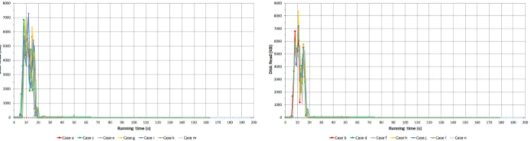
Figure 2 shows the utilization of disk capacity on N2 node. Similarly to cpu usage when the jobs are initiated usage of disk rises then it drops independently of the number of map processes and also some jumps occur at the end ofCases when map jobs are finished.
Figure 2: Speed of disk reading of N2
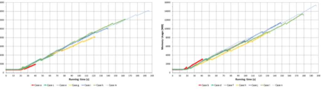
Figure 3: Size of reserved memory of N2
Figure 3 displays the memory usage of N2 node. Size of the reserved memory is independent of the number of initiated map processes.
4.1.2. Results in connection with the node where the “real” datanode is located
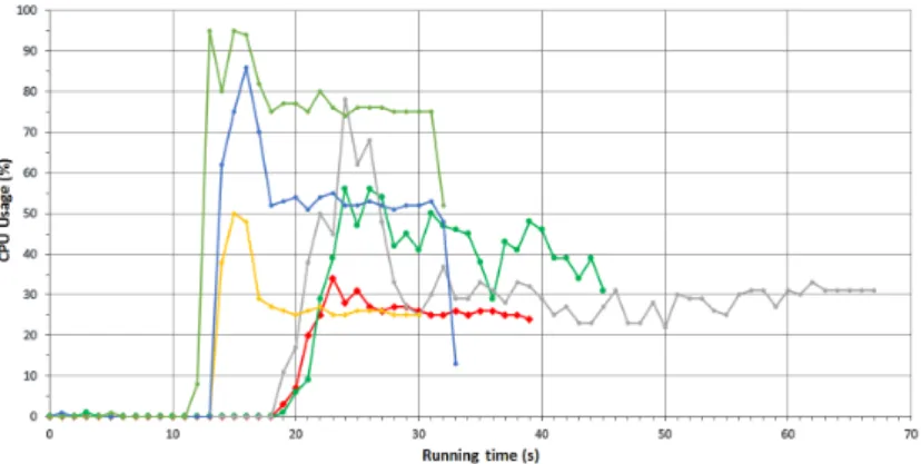
Figure 4: Cpu usage of N3
Figure 4 represents the cpu usage of N3 node. When one map is running (Case a) it reserves one of the four cores so cpu usage barely passes 25%. When two maps are running (Case b) it reserves two of the four cores so the maximum cpu usage can not step over 50% but it is around 40%. Whenever three or more maps are running simultaneously apart from the initial jump cpu usage stabilizes around
30%. The reason for this is the limit of disk reading capability as Figure 6 will prove that statement.
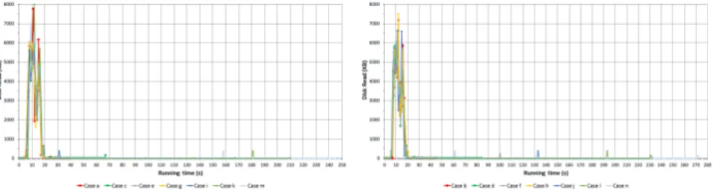
Figure 5: Speed of disk reading of N3
Figure 5 represents the utilization of capability of disk reading of N3 node.
In case of 1 map to read 1 GB it uses approximately the half of disk capability because only 1 core is reserved which is fully loaded.
When two maps are running two cpu cores are reserved and around 3/4 of disk capability is used. To read 2 GB into the memory lasts almost the same as in the first case but the speed of disk reading is almost twice as much as in Case a. Furthermore whenever three or more maps are running the limit of I/O arises because of the emerging congestion in the system. That is why cpu usage does not increase afterCase b.
Figure 6: Comparison of cpu usage
We investigate the scenario when we preload the necessary dataset into the memory so there is no I/O procedure during the running of the map tasks and the program reaches the data directly from the memory. From Figure 6 it can be observed when the data is reachable from the memory CPU usage reach the theoret- ical maximum in all Cases (Case_a_cache, Case_b_cache and Case_c_cache)
so it is clear that the cross section point is the I/O capability (reading).
Figure 7: Size of reserved memory of N3
Figure 7 shows the size of reserved memory of N3. As time goes by the amount of memory usage increases.
4.2. Scenario B
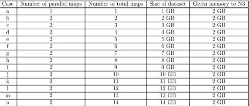
From the obtained results it appears that inCase a limit of cpu usage arises while in the other Cases limit of I/O capability restricts the performance. So in the next scenario the system is changed a little bit. Almost everything is the same as in Scenario A except that instead of 14 GB 2 GB RAM is given to yarn on N3 (see Table 4). This little modification has a remarkable effect on the operation of Hadoop, in Scenario B 2 maps can run in parallel at the same time altogether.
Case Number of parallel maps Number of total maps Size of dataset Given memory to N3
a 1 1 1 GB 2 GB
b 2 2 2 GB 2 GB
c 2 3 3 GB 2 GB
d 2 4 4 GB 2 GB
e 2 5 5 GB 2 GB
f 2 6 6 GB 2 GB
g 2 7 7 GB 2 GB
h 2 8 8 GB 2 GB
i 2 9 9 GB 2 GB
j 2 10 10 GB 2 GB
k 2 11 11 GB 2 GB
l 2 12 12 GB 2 GB
m 2 13 13 GB 2 GB
n 2 14 14 GB 2 GB
Table 4: Scenario B
Below (see Table 5) some results about running times can be noticeable, this table is the same as Table 3 with the results of Scenario B:
The same tendency takes place here as in Scenario B namely as more map processes are running in parallel the average processing time of 1 GB data starts to decrease then it remains around a constant value.
Running time Average running time of a map Initialization period Average processing time of 1 GB data
a 34 22 12 34 sec
b 48 36 12 24 sec
c 58 25 12 19.33 sec
d 68 28 12 17 sec
e 85 26,4 11 17 sec
f 92 26,1666667 12 15.33 sec
g 115 27 11 16.43 sec
h 126 28,5 11 15.75 sec
i 133 24,333 13 14.77 sec
j 142 25,5 11 14.2 sec
k 157 23,818181 13 14.27 sec
l 173 26,08333 13 14.42 sec
m 190 25,384615 12 14.62 sec
n 191 24,47143 13 13.64 sec
Table 5: Results in connection with running times
4.2.1. Results in connection with the node where AM is located As mentioned earlier the AM runs on this node on every occasion.
We use the same style as previously so the achieved results are divided into two groups according to the number of processed blocks:
∙ Number of processed blocks are odd (1,3,5,7,9,11,13)
∙ Number of processed blocks are even (2,4,6,8,10,12,14)
Figure 8: CPU usage of N2
On Figure 8 we can see the data of CPU usage of N2. We get back almost the same result as in Scenario A even the values are practically identical.
We can see the speed of disk reading of N2 on Figure 9. The situation is the same as in case of Scenario A. These figures also imply the fact that the little modification does not change the utilization of the resources of N2.
Figure 10 present the memory usage of N2. It is evident that the size of reserved memory depends a little on the number of launched map processes.
4.2.2. Results in connection with the node where the “real” datanode is located
Figure 11 demonstrates the CPU usage of N3. It is noticeable that in particular intervals the CPU usage boosts. These phenomena can by explained by the fact
Figure 9: Speed of disk reading of N2
Figure 10: Size of reserved memory of N2
Figure 11: CPU usage of N3
that 2 map processes can run in parallel at the same time so when 3 GB or more data are processed launching a new map process requires some time. In these intervals the CPU usage is greater. Another interesting situation is observable in cases of odd numbered processed blocks because at the end of the running of the last map process CPU usage decreases to about 25% as only one map is running at that time.
Figure 12 shows the speed of disk reading of N3. The same tendency can be observed as in CPU usage. Here we reserve less resources compare to the other scenario. Just 2 maps can run at the same time in parallel so the factor of congestion is smaller but we do lose some time whenever a map finishes/starts. Despite that fact it still results greater speed of disk reading in overall compared to Scenario A.
Figure 12: Speed of disk reading of N3
Figure 13: Comparison of cpu usage
Figure 13 presents the situation when the necessary dataset is available from memory. The difference is still there among the appropriateCases (like between Case b andCase_b_cache orCase c andCase_c_cache) but it is smaller than in Scenario A.
Figure 14: Size of reserved memory of N3
Figure 14 show the size of reserved memory of N3. As time goes by the amount
of memory usage increases.
Let introduce the following notations:
∙ n(t): at time𝑡the number of parallelly running maps
∙ T: entire running time of the map in seconds
∙ g: the cost of required resource of one map
∙ K: the cost of the entire running time
Then ∑︁𝑇
𝑡=0
(𝑔*𝑛(𝑡)).
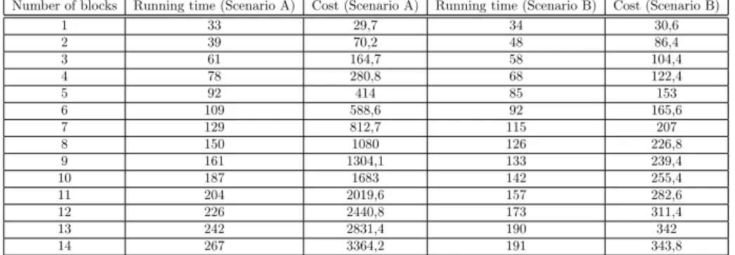
In the Table 6 we used the following formula: 𝐾 = 𝑇 *𝑛*𝑔, where n is the maximum number of executable maps.
The next table compares the investigated scenarios where𝑔= 0.9:
∙ We gave 14 GB memory to YARN so the whole dataset can be executable in parallel. The number of parallelly executable maps are 14 (MAP14).
∙ We gave 2 GB memory to YARN. The number of parallelly executable maps are 2 (MAP2).
Number of blocks Running time (Scenario A) Cost (Scenario A) Running time (Scenario B) Cost (Scenario B)
1 33 29,7 34 30,6
2 39 70,2 48 86,4
3 61 164,7 58 104,4
4 78 280,8 68 122,4
5 92 414 85 153
6 109 588,6 92 165,6
7 129 812,7 115 207
8 150 1080 126 226,8
9 161 1304,1 133 239,4
10 187 1683 142 255,4
11 204 2019,6 157 282,6
12 226 2440,8 173 311,4
13 242 2831,4 190 342
14 267 3364,2 191 343,8
Table 6: Comparison of the scenarios
5. Conclusion
This paper addressed optimization techniques for reducing the time-consumption and computational resource usage in a Hadoop cluster. Running time, CPU us- age, memory usage, and Speed of disk reading of the nodes are the subjects that have been screened in the Hadoop cluster to examine the proposed optimization techniques for searching the frequency of DNA signatures (k-mers) in the genomic
data. The obtained results show that using all the resources (CPU, memory) is not always the best solution and our scenarios is a prime example of it. Managing the maps according to the size of data and memory is critical. Our results also indicate that the speed of I/O greatly affects the effectiveness of performance. To get a better and faster operation, optimizing the configurations and parameters of Hadoop is also required in order to reduce the data transfer and communication between nodes of the cluster. Comparing two Scenarios show another remarkable result; running the maps in parallel causes shorter processing time. The aim of this research is to enhance the possibility of using ordinary computers as a distributed computing system for the entire research community to analyze large-scale dataset.
References
[1] L. Barzon,E. Lavezzo,V. Militello,S. Toppo,G. Palù:Applications of Next-Genera- tion Sequencing Technologies to Diagnostic Virology, International Journal of Molecular Sciences 12.11 (2011), pp. 7861–7884,doi:10.3390/ijms12117861.
[2] C. X. Chan,M. A. Ragan:Next-generation phylogenomics, Biology Direct 8.3 (2013),doi:
10.1186/1745-6150-8-3.
[3] J. Dean,S. Ghemawat:MapReduce: Simplified Data Processing on Large Clusters, Com- munications of the ACM 51.1 (2008), pp. 107–113,doi:10.1145/1327452.1327492.
[4] M. Domazet-Lošo,B. Haubold:Alignment-free detection of local similarity among vi- ral and bacterial genomes. Bioinformatics. 27.11 (2011), pp. 1466–1472, doi: 10 . 1093 / bioinformatics/btr176.
[5] J. A. Gilbert,C. L. Dupont:Microbial metagenomics: beyond the genome.Annual review of marine science. 3 (2011), pp. 347–371,doi:10.1146/annurev-marine-120709-142811.
[6] J. Handelsmanl,M. R. Rondon,S. F. Brady,J. Clardy,R. M. Goodman:Molecu- lar biological access to the chemistry of unknown soil microbes: a new frontier for natural products.Chemistry & biology 5.10 (1998), R245–R249.
[7] B. Haubold,F. Reed,P. Pfaffelhuber:Alignment-free estimation of nucleotide diver- sity, PLOS Computational Biology 27.4 (2011), pp. 449–455,doi:10.1093/bioinformatics/
btq689.
[8] Human Genome Project,https://web.ornl.gov/sci/techresources/Human_Genome/index.
shtml.
[9] R. Karimi,L. Bellatreche,P. Girard,A. Boukorca,A. Hajdu:BINOS4DNA: Bitmap Indexes and NoSQL for Identifying Species with DNA Signatures through Metagenomics Samples, in: Information Technology in Bio- and Medical Informatics, Switzerland: Springer, Cham, 2014, pp. 1–14,doi:10.1007/978-3-319-10265-8_1.
[10] R. Karimi, A. Hajdu: HTSFinder: Powerful Pipeline of DNA Signature Discovery by Parallel and Distributed Computing, Evolutionary bioinformatics online 12 (2016), pp. 73–
85,doi:10.4137/EBO.S35545.
[11] C. Kemena,C. Notredame:Upcoming challenges for multiple sequence alignment methods in the high-throughput era. Bioinformatics. 25.19 (2009), pp. 2455–2465, doi: 10 . 1093 / bioinformatics/btp452.
[12] S. Moorthie, C. J. Mattocks,C. F. Wright:Review of massively parallel DNA se- quencing technologies, The HUGO journal 5.1-4 (2011), pp. 1–12, doi:10.1007/s11568- 011-9156-3.
[13] C. S. Pareek,R. Smoczynski,A. Tretyn:Sequencing technologies and genome sequenc- ing.Journal of applied genetics. 52.4 (2011), pp. 413–435,doi:10.1007/s13353-011-0057-x.
[14] E. Pettersson,J. Lundeberg,A. Ahmadian:Generations of sequencing technologies.
Genomics. 94.2 (2009), pp. 105–111,doi:10.1016/j.ygeno.2008.10.003.
[15] T. Thomas,J. Gilbert,F. Meyer:Metagenomics - a guide from sampling to data anal- ysis, Microbial Informatics and Experimentation 2.3 (2012),doi:10.1186/2042-5783-2-3.
[16] T. J. Treangen,S. L. Salzberg:Repetitive DNA and next-generation sequencing: com- putational challenges and solutions.Nature reviews. Genetics. 13.1 (2011), pp. 36–46,doi:
10.1038/nrg3117.
[17] K. V. Voelkerding,S. A. Dames,J. D. Durtschi:Next-generation sequencing: from basic research to diagnostics.Clinical chemistry. 55.4 (2009), pp. 641–658, doi:10.1373/
clinchem.2008.112789.
[18] T. White:Hadoop: The Definitive Guide, Sebastopol, California, USA: O’Reilly Media, 2015.
[19] J. C. Wooley,A. Godzik,I. Friedberg:A Primer on Metagenomics, PLOS Computa- tional Biology 6.2 (2010),doi:10.1371/journal.pcbi.1000667.
[20] J. Zhang,R. Chiodini,A. Badr,G. Zhang:The impact of next-generation sequencing on genomics, J Genet Genomics. 38.3 (2011), pp. 95–109,doi:10.1016/j.jgg.2011.02.003.