USING THE STATED PREFERENCE METHOD FOR THE CALCULATION OF SOCIAL DISCOUNT RATE1
Andrea Tabi
Department of Environmental Economics and Technology, Corvinus University of Budapest E-mail: andrea.tabi@uni-corvinus.hu
The aim of this paper is to build the stated preference method into the social discount rate methodology. The first part of the paper presents the results of a survey about stated time preferences through pair-choice decision situations for various topics and time horizons. It is assumed that stated time preferences differ from calculated time preferences and that the extent of stated rates depends on the time period, and on how much respondents are financially and emotionally involved in the transactions. A significant question remains: how can the gap between the calculation and the results of surveys be resolved, and how can the real time preferences of individuals be interpreted using a social time preference rate. The second part of the paper estimates the social time preference rate for Hungary using the results of the survey, while paying special attention to the pure time preference component.
The results suggest that the current method of calculation of the pure time preference rate does not reflect the real attitudes of individuals towards future generations.
Keywords: social discount rate, stated preferences, revealed preferences, cost-benefit analysis JEL codes: D90, D91
1. Introduction
The long term impacts of climate change, losses of biodiversity and a decrease in available freshwater will sporadically impact different areas of the Earth, rendering evaluation of such events more difficult and also increasing the role of uncertainty when calculating social investment.
1 The research described herein was financed by the following grant: OTKA105228.
1
There are many evaluation methods which address environmental impacts. One of these methods is cost-benefit analysis (CBA) which is designed to monetize all goods and services (including non-marketed goods as well), thereby helping decision-makers decide which project or program has the highest value or utility to society. CBA can be carried out on the micro or macro level and in most cases, depending on the lifespan of the project assessed, it is necessary to model future scenarios (Höjer et al. 2008). In order to calculate the net present value of the future societal costs and benefits, assumptions regarding prices and attitudes must be made, not only for the determination of costs and benefits, but for the social discount rate.
The social discount rate is designed to capture in one parameter how the wellbeing of future generations is discounted by the present generation. As such, it is also one of the most crucial elements of CBA. A lot of factors must be considered in the evaluation by current generations, such as the risk of uncertainty, impatience, myopia, altruism, etc. Thus, during the calculation of the social discount rate it is necessary to make a decision about how to weight these factors.
This paper analyzes and validates the currently used methodology for calculating the social discount rate and also points out its weaknesses and crucial theoretical points, which need to be considered in the future in order to get closer to more reliable estimations.
In the first part of this paper the social discount rates is measured using stated preference methodology. The survey is based on a representative sample of 1,000 people, carried out in Hungary in 2010. Besides the rates obtained in the survey, relationship analysis was conducted on time preference questions and other variables such as gender, age, attitudes, happiness etc., in order to determine which factors have the largest influence on time discounting behavior.
Secondly, assuming that stated preferences are suitable for validating the parameters used in the calculation of the social discount rate, social time preference rate (STPR) methodology is tested whether it fits for purpose or not, paying special attention to the pure time preference rate. The hypothesis is that the current definition and calculation method for the pure time preference component does not reflect the real preferences of individuals towards future generations.
2
2. Overview of the literature overview – A short introduction into social discounting Difficulties are caused by the abstraction of long term social discounting because it tries to capture the social decision-making algorithm of an event with consequences which take place in the (sometimes) distant future. Because of personal involvement, the time period is usually determined by the individuals’ lifespan and not by the impacts of activity in question.
Therefore two sorts of discounting have to be distinguished according to time horizon: intra- and intergenerational discounting. The latter is considered to be a long term discounting method.
There are basically three different approaches utilized with temporal discounting patterns, based on the calculation methodology for the social discount rate: normative, revealed and stated preferences. The normative approach determines the value of the discount rate only using ethical considerations. The literature which considers ethical disputes as grounds for discounting (and the question of whether the wellbeing of the next generations can be discounted at all) may be divided into two streams: the first stream contains research which considers only a zero rate to be ethically appropriate (e.g. Ramsey 1928; Pigou 1932; Broome 1992; O’Neill 1993; Norgaard – Howarth 1991), because any positive rate is non-neutral from the perspective of intergenerational equality. The other stream suggests a negative discount rate in order to revalue the next generations altruistically (e.g. Loewenstein – Prelec 1992).
The revealed preference approach examines temporal discounting behavior from a top-down perspective, utilizing macro data. This method typically captures consumer behavior (i.e.
behavior of a certain group of people). The main difference between revealed and stated preferences is that the revealed preference method can only be used to appraise decisions about marketable goods, while in contrast stated preference methods can capture both marketable and non-marketable values as well (Ahlroth – Finnveden 2011). The calculation of the social time preference rate is mainly based on the revealed preferences of the government and individuals. The equation for social time preference rate, first suggested by Ramsey (1928) is the following:
STPR = p + eg (1)
The first part is the pure time preference rate (p), which describes people’s attitudes to the welfare of future generations. The second part makes the next generations’ welfare equal with 3
the current generation’s welfare. This part is calculated from the product of two parameters:
elasticity of marginal utility of consumption (e) and the growth rate of per capita real consumption (g) (Evans – Sezer 2005). There are several methods for calculating each parameter, but most prevalent is a tax-based (mostly income tax) method for capturing the elasticity of the marginal utility of consumption (Evans 2005) and the use of GDP as growth rate.
From an ethical point of view, a pure time preference rate is problematic, and this is addressed through a very wide spectrum of theories. The use of zero, negative and positive rates have been suggested; disputes usually concern the same issues as mentioned above. Arguments for positive rates usually refer to myopia and the impatience of individuals. Dasgupta and Maskin (2005) claimed that preferences are manifested in urges, cravings, and inclinations which are the consequences of our evolutionary development. Benefit-maximizing behavior is thus a typical problem for decision theory.
Stated preferences directly describe individuals’ choices about future rewards or costs through the use of a survey-based methodology which belongs to realm of choice modeling (Pearce et al. 2006). There are two techniques; one typical approach is a paired comparison exercise where respondents are asked to choose one preferred alternative out of two options regarding a given time horizon. These types of questions are usually arranged on an ordinal scale. The other way of investigating time preferences is to use open questions where respondents have to make choices. Willingness to complete open questions is lower, but provides more reliable results. Similar empirical research (Loewenstein – Prelec 1992; Chapman 1996, Lazaro et al.
2002) has documented that the discount rates derived from stated preference approaches are much higher than those derived from revealed preference approaches, based on demographic and macro data.
The same research highlights the fact that discount rates are not constant over time, but decrease and can be described using a hyperbolic curve. Until recent times, Samuelson’s discounted utility model (introduced in 1937) was applied to the CBA of and was generally accepted as a model capable of describing actual intertemporal behavior. However, the observed anomalies in responses showed that individuals’ actual discounting behavior is not exponential – as Samuelson’s model suggests. The anomalies are claimed to be the following (Loewenstein – Prelec 1992): a sign effect (gains are discounted more than losses); a
4
magnitude effect (small amounts are discounted more than large amounts); a delay/speed-up asymmetry (greater discounting is shown to avoid delay of a good than to expedite its receipt); improving sequences (in choices over sequences of outcomes, improving sequences are often preferred to declining sequences though positive time preference dictates the opposite); violations of independence and preference for spread (in choices over sequences, violations of independence are pervasive, and people seem to prefer spreading consumption over time). Beyond those anomalies, a time effect (an inverse relationship between time horizon and discount rates) and domain effects (different discount rates are used for different goods; e.g., money, health) can be observed in the case of long-term stated time preferences (Chapman 1996). Chapman (2001), Lazaro et al. (2002) and Berndsen and Pligt (2001) conducted studies on students and revealed their time preferences for various topics. Lazaro et al. (2002) found that stated preferences do not correspond with the behavior predicted by the axioms of Samuelson’s discounted utility model and their results also underpin the assumptions of the time effect, the magnitude effect and the delay / speed-up asymmetry in social intertemporal decisions.
Chapman (2001) undertook three experiments using a sample of students and studied the difference between intergenerational and intragenerational discounting behavior. Despite the assumption that the intergenerational discount rates would be lower, empirical research showed similar parameters for both time intervals.
Svenson and Karlsson (1989) as well as Hendrickx and Nicolaij (2004) investigated the connection of temporal discounting with environmental risk. Hendrickx and Nicolaij (2004) focused on ethical and loss-relating concerns related to risk evaluation. Svenson and Karlsson (1989) analyzed the significance of time horizons and the discounting of negative consequences using a decision theory framework. Both empirical studies found that the majority of people discount environmental risks less than other risks. Such differences emphasize the role of ethical concerns in risk evaluation.
In contrast to these results Hardisty and Weber (2009) found that individuals discount environmental outcomes in a similar manner to how they discount financial outcomes using short to medium delays (1 to 10 years). They examined three domains: hypothetical financial, environmental and health gains and losses. Only health losses were discounted less than the other two domains.
5
Kula and Evans (2011) suggest the use of a dual discounting method, which implies the separation of environmental benefits from other costs and benefits. Thus, in theory, dual discounting can contribute to the realization of more environmentally-friendly projects.
Figure 1. Comparison of different discounting methods (discount rate 3,5%)
Figure 1 illustrates four different discounting methods. The exponential function as the conventional method and hyperbolic discounting have already been discussed. ‘Green Book’
refers to the time-declining rates used in the HM Treasury guideline (2003) in the UK which suggests various discount rates which decline over time (Pearce et al. 2006). This type of discounting basically does not differ from the exponential function. The Modified Discount Factor (MDF) introduced by Kula (2006) assumes that the size of the society and the life expectancy of individuals are constant throughout and it takes the distant consequences of a project into account; i.e. the discount factor does not converge to zero over time.
3. Survey
0 0,1 0,2 0,3 0,4 0,5 0,6 0,7 0,8 0,9 1
1 8 15 22 29 36 43 50 57 64 71 78 85 92 99 106 113 120 127 134 141 148 155 162 169 176 183 190 197
Discount factor
Years
Green Book Exponential Hyperbolic MDF
6
The results presented herein are based on a survey which used a representative sample of 1,000 people, which contrasts with research done by other authors (such as Chapman 1996;
Lazaro et al. 2002) who undertook research using samples of students. It is considered that students do not represent the actual attitudes of all social clusters, although they may provide accurate answers. This survey is representative of the Hungarian population regarding gender, age and income.
The questions in the survey were designed to measure personal preferences to receiving rewards in the future, and were also designed to capture the personal preferences which concern common decisions – mainly through allocation of common costs over time. The methodology was also designed to reveal long term intergenerational time preferences through ‘saving lives’. The last set of questions investigated people’s willingness to pay (WTP) the future costs of climate change.
3.1. Methods
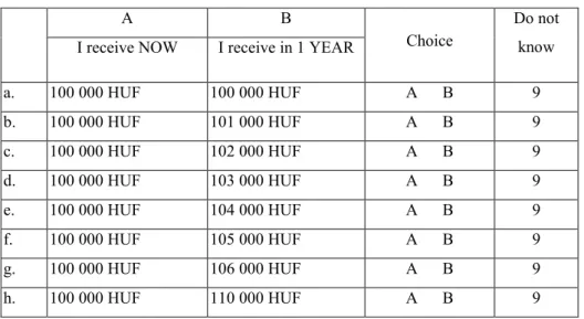
Each questionnaire consisted of 4 types of questions and each question type contained 11 pairs of 2 alternatives arranged on an ordinal scale. Thus it was possible to investigate respondents’ “switching points” – where they switched from alternative “A” to alternative
“B”. For example, the first type of question assumes a hypothetical situation where the respondent wins a certain amount of money and has to decide when he/she wants to receive it.
Alternative “A” involves receiving 100,000 HUF immediately while alternative “B” involved receiving a larger amount 1 year later.
Table 1. Sample question: Winning money now or with 1 year delay?
A B
Choice Do not know I receive NOW I receive in 1 YEAR
a. 100 000 HUF 100 000 HUF A B 9
b. 100 000 HUF 101 000 HUF A B 9
c. 100 000 HUF 102 000 HUF A B 9
d. 100 000 HUF 103 000 HUF A B 9
e. 100 000 HUF 104 000 HUF A B 9
f. 100 000 HUF 105 000 HUF A B 9
g. 100 000 HUF 106 000 HUF A B 9
h. 100 000 HUF 110 000 HUF A B 9
7
i. 100 000 HUF 115 000 HUF A B 9
j. 100 000 HUF 120 000 HUF A B 9
k. 100 000 HUF 125 000 HUF A B 9
Note: 277 HUF/EUR was the average exchange rate in May 2010.
The second type of question referred to social decisions related to flood protection. The hypothetical situation was as follows: “Imagine that the state offers a certain amount of money to villages along the river Tisza which has to be spent on flood protection. If the subsidy is asked for immediately, the state will offer a lower amount; however, if you wait 1 or 10 years, villages will get a larger sum which makes more efficient protection possible (e.g., stronger dams). What is your decision?” The purpose of this question is to reveal people’s attitudes to urgent and pressing situations where it is important to act as soon as possible. Our assumption is that in such a decision situation, where intervention is urgent, using time preference rates is meaningless and using stated preferences will lead to a paradox exchange: the quicker the intervention should be the higher the time preference rate, which induces the postponing of action.
The third type of question deals with saving lives using the following hypothetical situation:
“Imagine that you have to decide between two programs of financial support for medicine and therapy research. In Program “A”, a pre-existing treatment is supported which can save 100 lives immediately. Program “B” supports medical research which could help more than 100 people in 1, 30 or 100 years to stay alive. What is your decision?”
The last group of questions, regarded as the most abstract or hypothetical, dealt with the financial consequences of climate change: “Imagine that you have to choose from two options regarding climate costs. Option “A” is that from now on you pay a certain amount annually (to cover the costs of climate change), and option “B” involves postponing the costs and paying 1 million HUF (in 10 years) or 10 million HUF (in 30 years) when the catastrophic consequences of climate change occur. What is your decision?”
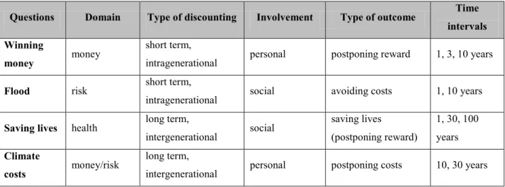
In all cases, inflation is ignored: 1 HUF now is equal to 1 HUF in the future. Table 2 summarizes the four types of questions by temporality, involvement, type of outcome, and time horizon.
8
Table 2. Types of questions
Questions Domain Type of discounting Involvement Type of outcome Time intervals Winning
money money short term,
intragenerational personal postponing reward 1, 3, 10 years
Flood risk short term,
intragenerational social avoiding costs 1, 10 years Saving lives health long term,
intergenerational social saving lives
(postponing reward)
1, 30, 100 years Climate
costs money/risk long term,
intergenerational personal postponing costs 10, 30 years
Discount rates were calculated using to the following equation:
𝐷𝑖𝑠𝑐𝑜𝑢𝑛𝑡 𝑟𝑎𝑡𝑒 = �𝑖𝑛𝑑𝑖𝑓𝑓𝑒𝑟𝑒𝑛𝑐𝑒 𝑝𝑜𝑖𝑛𝑡 𝑖𝑚𝑚𝑖𝑑𝑖𝑎𝑡𝑒 𝑏𝑒𝑛𝑒𝑓𝑖𝑡�
1
𝑛 − 1 (2)
where n is the number of years implied in the choice. The indifference point is the point where the respondent switches from one alternative to some other (Chapman 2001). The indifference number is indicated by the last preferred immediate benefit (alternative “A”), before alternative “B” is chosen (e.g. if winning 115,000 HUF in 1 year is preferred to 100,000 HUF now, but 100,000 HUF now is preferred to getting 110,000 HUF in 1 year, then the indifference point is 110,000 HUF).
In the questionnaire, respondents were also asked about their happiness, life satisfaction, general attitude to the environment (5 questions) and personal data (gender, age, number of children, qualification, net income).
3.2. Results
Although 1,012 individuals completed the questionnaire, some values were missing, and in many cases the results were not appropriate for analysis for different reasons. It often occurred that respondents chose two or more switching points which were not consistent with an ordinal scale, or they did not switch from one alternative to another. The latter could have happened for several reasons: (1) respondents did not want to discount at all; (2) the scale was not wide enough, thus they could not find their indifference point; (3) respondents did not 9
understand the situation; or, (4) they did not want to make a decision. Inconsistent and unusable replies were coded “do not know” and excluded from further analysis. The majority of respondents marking the option “choosing now” and were also excluded from the further calculations because it was not clear that the rates are either higher than the maximum value of the given table or they do not want to discount at all.
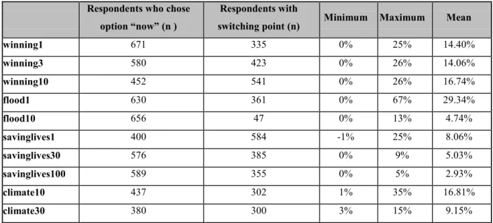
Table 3 shows the number of respondents, the minimum and maximum values for discount rates and the statistical means, by questions. Time delays were designed to be different because of the various topics and level of respondent involvement. A repeated measurement analysis of variance (RM ANOVA) was conducted between time delays within each question group. The results of the RM ANOVA suggest that the time delays within all question groups significantly differ from each other (Greenhouse-Geisser and Huynh-Feldt tests show p=0.000 significance level), but according to the pairwise comparisons of means using the Bonferroni correction for the “winning money” scenario, the means of the time delays of 1 and 3 years do not differ statistically (p = 0.546).
Table 3. Average discount rates by question
Respondents who chose option “now” (n )
Respondents with
switching point (n) Minimum Maximum Mean
winning1 671 335 0% 25% 14.40%
winning3 580 423 0% 26% 14.06%
winning10 452 541 0% 26% 16.74%
flood1 630 361 0% 67% 29.34%
flood10 656 47 0% 13% 4.74%
savinglives1 400 584 -1% 25% 8.06%
savinglives30 576 385 0% 9% 5.03%
savinglives100 589 355 0% 5% 2.93%
climate10 437 302 1% 35% 16.81%
climate30 380 300 3% 15% 9.15%
In the ‘Saving lives’ and ‘Climate costs’ scenarios long-term (intergenerational) discount rates were uncovered, and it is observable that these rates fall as the delay increases (time effect).
There is, additionally, a significant difference between discounting money and health (domain effect). The high rates for flood protection with a 1-year delay imply a preference for early intervention and the very low number of responses in favor of a 10-year delay also
10
corresponds with the findings of Svenson and Karlsson (1989) as well as Hendrickx and Nicolaij (2004), illustrating that the majority of people do not discount environmental risks or they cannot make a decision about the extent of delays and rewards. A flood with a 1-year delay induces the highest rates, while only 47 people chose the 10 year delay. This question is designed to test people’s attitudes towards environmental issues where they could be personally affected.2 Responses to the questions concerning flood protection are, because of the high standard deviation, excluded from the further analysis.
The fourth question type is practically a WTP design. Respondents were asked about when and how they would pay to avoid damages caused by climate change. Two-thirds of respondents wanted to pay from now on annually in both time intervals and approximately 10-15% of respondents to pay the damages of climate change 10 or 30 years later.
A one-way ANOVA procedure was conducted for each question group using discount rates as dependent variables. Independent variables were gender, age, net income, qualification, happiness, life satisfaction, number of children and environmental attitude questions. No connection could be observed between time discounting and gender: women and men use the same discount rates. There was no correlation observed between time discounting behavior and age groups or the number of children, which suggests that elderly people discount the future in the same way as younger people, and also that young people consider their future as serious as elderly people. In the cases of happiness and life satisfaction discount rates do not differ and associated standard deviations are also very small, so not surprisingly no significant connection was found with time preferences. Three variables proved to be significantly correlated with time discounting behavior: household net income, qualification and environmental attitudes. Net income and qualifications were compared in the two major domains, money and health.
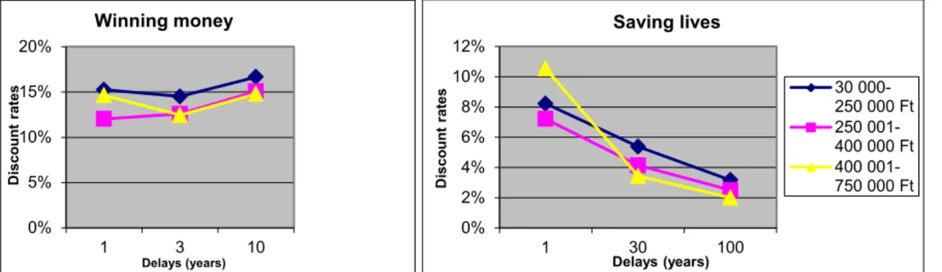
In the case of ‘winning money’, the discount rates of income groups for respondents who chose a 1 year delay differ from each other (p=0.027); the same is found for a 3 year delay (p=0.194) and a 10 year delay (p=0.209). Discount rates increase over time; namely, rates with 10 year delay are higher than for a 1 year delay. The highest rates can be observed in the
2 In Hungary, flood protection is unfortunately an annually recurring problem and a lot of towns along the Tisza river are threatened by floods. So far, a huge amount of money has been spent by the government on damns and compensations, thus the sensitivity of individuals in Hungary is quite high to this particular issue.
11
lowest income group in every time interval, but the highest income category cannot be unambiguously separated from the other two groups.
Figure 2. Comparison of domains ‘health’ and ‘money’ by income groups
The discount rates for health-related outcomes significantly differ from each other and from other domains as well. Health was discounted the least of all domains. A statistically significant difference is found for income levels for the 30 year (p=0.005) and 100 year (p=0.011) delays, while for 1 year no such correlation was found (p=0.537).
Figure 3. Comparison of domains ‘health’ and ‘money’ by qualification
Figure 3 shows the average discount rates compared with level of education. In our sample the majority of respondents did not graduate from high school (mostly skilled worker), are middle aged, and are in the middle income category. Skilled workers who did not attend high school used the highest rates in both cases. The discount rates of respondents with a university degree show a linear curve; these respondents used almost the same rates for each delay regarding money, and discount rates decrease from 4.8% to 3.27% in the ‘Saving lives’
domain. A significant difference can be observed for ‘Winning money’ at 1 (p=0.003), 3 year
0%
5%
10%
15%
20%
1 3 10
Discount rates
Delays (years)
Winning money
0%
2%
4%
6%
8%
10%
12%
1 30 100
Discount rates
Delays (years)
Saving lives
30 000- 250 000 Ft 250 001- 400 000 Ft 400 001- 750 000 Ft
0%
2%
4%
6%
8%
10%
1 30 100
Discount rates
Delays (years)
Saving lives
0%
10%
20%
1 3 10
Discount rates
Delays (years)
Winning money
skilled workers, high school without graduation
high school graduation
accredited training after graduation, college
12
(p=0.001), and 10 year (p=0.113) delays, where the p-values also show some variation. In the Saving Lives domain the rates statistically differ from each other with a 30 year delay (p=0.080) for a 1 year (p=0.211) and 100 year (p=0.168) delay.
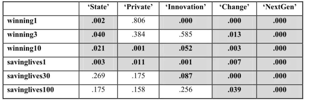
General attitude questions towards the environment were also asked in order to reveal how people evaluate the environment and what they think should be done to preserve natural resources for the next generation. Respondents were asked to decide using a 5-grade scale (1 – totally disagree, 5 – totally agree) whether they agree or disagree with the following statements:
1. The state is responsible for preserving our natural resources. (‘State’)
2. It is everybody’s right to use natural resources for private purposes. (‘Private’)
3. I believe that technological development and innovation will solve environmental problems. (‘Innovation’)
4. We should radically change our consumption behavior in order to preserve our environment. (‘Change’)
5. People must ensure that natural resources will be available for the next generations.
(‘NextGen’)
As shown in Table 4, responses to these questions indicate a very strong relationship between attitudes to environment/next generations and time preferences – or at least significant differences between subgroups. In the case of the last two statements (‘Change’/’NextGen’) discount rates proved to be significantly different to each other in the 5 subgroups. Detailed analysis of this finding is now presented.
Table 4. One-way ANOVA for variables (sig. levels, p<0.1)
‘State’ ‘Private’ ‘Innovation’ ‘Change’ ‘NextGen’
winning1 .002 .806 .000 .000 .000
winning3 .040 .384 .585 .013 .000
winning10 .021 .001 .052 .003 .000
savinglives1 .003 .011 .001 .007 .000
savinglives30 .269 .175 .087 .000 .000
savinglives100 .175 .158 .256 .039 .000
4. Calculating the pure time preference rate
13
The pure time preference rate is the most crucial element when defining STPR. Many authors have tried to determine its actual value using both empirical and theoretical methods, but there is still no universally accepted agreement on this topic.
Authors such as Ramsey, Broome and Pigou consider the zero rate to be ethically indefensible (regarding future generations). Broome (1991) argues for impartiality towards current and future generations, which means that there should be no difference between the wellbeing of society today or in the future thus no discounting should be applied; in other words, the discount rate must be zero. The concept of utilitarianism may also be employed to argue for the use of a zero rate (Pearce 1995). If it is considered that future generations will be better off than the current one – assuming capital accumulation and technical development – a zero discount rate can contribute to the efficient allocation of resources across generations. The use of a zero discount rate can thus be underpinned by ethical theory (impartiality) and also the correct redistribution between generations weighting the one that will be better off.
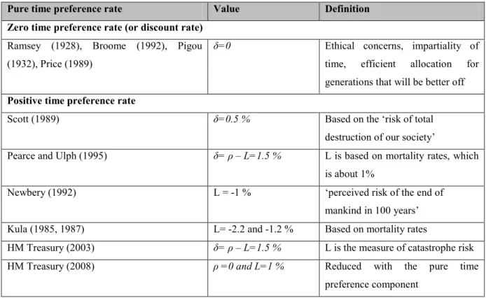
Positive pure time preference rates are explained by myopia and the impatience of individuals (Evans 2006). On the basis of several studies a positive value in the range of 0.5-2% is suggested – mostly based on mortality rates (see Table 5).
Table 5. Estimates of pure time preference rate
Pure time preference rate Value Definition
Zero time preference rate (or discount rate) Ramsey (1928), Broome (1992), Pigou (1932), Price (1989)
δ=0 Ethical concerns, impartiality of
time, efficient allocation for generations that will be better off Positive time preference rate
Scott (1989) δ=0.5 % Based on the ‘risk of total
destruction of our society’
Pearce and Ulph (1995) δ= ρ – L=1.5 % L is based on mortality rates, which is about 1%
Newbery (1992) L = -1 % ‘perceived risk of the end of
mankind in 100 years’
Kula (1985, 1987) L= -2.2 and -1.2 % Based on mortality rates
HM Treasury (2003) δ= ρ – L=1.5 % L is the measure of catastrophe risk
HM Treasury (2008) ρ =0 and L=1 % Reduced with the pure time
preference component
14
Source: Pearce and Ulph (1995) and Evans (2006)
In order to quantify this parameter better, Pearce and Ulph (1995) developed the Ramsey formula with an additional element. L (changing life chances) which expresses changing risks to life. This is calculated from the ratio of mortality to population (mortality rate). L takes a negative value so it can be added to the pure time preference rate: thus if life chances increase, the social discount rate will decrease. The idea behind using the mortality rate is the assumption that life risks are increasing over time. However, using the mortality rate creates several problems as described by Pearce and Ulph (1995), e.g. in case of a very long-term project the increasing probability of death of an individual does not play a role. In intergenerational discounting the life chances of the whole population are important, not risks occurring at an individual level. There are several further theoretical reasons in opposition to using the death rate: the idea that people ‘smooth out’ their consumption over a lifetime is underpinned by the ongoing development of medical treatments and by noting the social benefits provided by the state to the elderly (pension, disability aid, etc.). Preferring early consumption over later is not always a consequence of the increasing chance of death. For instance, elderly people often consume less in order to save up money to help their children or grandchildren, thus consumption may decrease over time, but not for reasons of mortality. To sum up, assessing the distribution of consumption over an individual’s lifetime is complex and care must be taken to avoid painting an inappropriate picture of people’s attitudes towards future generations.
Besides theoretical arguments, the use of mortality rate as an expression of people’s attitudes is distinctly refuted by the empirical results as well. According to the sample, ageing has no connection with discounting behavior; elderly people discount in the same way as young people do.
L was adapted as a measure of the pure time preference rate by the EU Guide to Cost-Benefit Analysis (2008) and in the Green Book (2003) in the United Kingdom (although the latter changed meaning so that L became the risk of a catastrophe, meaning the likelihood of natural disasters/wars that can dramatically alter our environment). The effort to expand the meaning of L to a more intergenerational level raises the problem of reliability. Calculations regarding the probability of unforeseeable events happening in 50 or 100 years lead us to different future scenarios with totally different consequences. Let us take the example of a nuclear war
15
that can considerably alter and devastate a whole country. If we accept the possibility of a nuclear war happening in the near future, then there is no point in initiating social or environmental projects and the social discount rate should be very high. Natural disasters are more predictable and when they happen more frequently in the course of time, according to our empirical results, people do not discount but rather prefer immediate intervention.
Accordingly, for projects or programs concerning the avoidance or amelioration of urgent situations (such as the threats of flood) the pure time preference rate should be zero.
Empirical evidence indicates that time preferences are most influenced by attitude. During analysis of the survey it became clear that rates differ from each other by domain and time intervals as well. From the five attitude questions the one regarding innovation was the most divisive, although subgroups were not significantly different for every time preference question. Table 6 shows the average rates using the 5-grade scale in the ‘Saving Lives’
domain.
Table 6. Discount rates by attitude question (innovation)
‘Innovation’ lifesaving1 lifesaving30 lifesaving100
Totally disagree Mean 3.76% 4.28% 2.92%
N 38 18 13
2 Mean 8.23% 4.81% 2.47%
N 69 47 43
3 Mean 6.58% 4.78% 2.90%
N 212 132 123
4 Mean 9.43% 5.16% 3.14%
N 174 122 114
Totally agree Mean 10.12% 5.95% 3.05%
N 78 59 56
Total Mean 7.94% 5.06% 2.95%
N 571 378 349
It can be seen that the pure time preference rate corresponds to people’s attitudes to future generations, so the ‘Saving Lives’ questions (over the very long term) can serve as a proxy for the theoretical parameter (δ) described above. According to the empirical results a pure time preference rate in the range of 0-2 % seems acceptable using a 100 year time interval.
16
If the reasoning for using a positive pure time preference rate is accepted, then the range of 0.5-2% suggested by the top-down methods largely corresponds to the results derived from stated preference surveys.
5. The calculation of STPR for Hungary
As already described, the social time preference rate is composed of the pure time preference rate (p) and a second part (eg) which makes the utility of generations equal. The EU Guide to Cost-Benefit Analysis suggests a tax-based calculation (Stern 1977) for the marginal elasticity of consumption (e) and GDP growth for the growth rate (g).
The most popular approach to calculating the e parameter is based on tax structure (mostly on income taxes). It is designed to mirror state taxation policy aimed at smoothing out income inequalities. Thus the more progressive the income tax structure, the higher the value of e.
The following relationship is based on the iso-elastic utility function and the principle of equal absolute sacrifice of satisfaction developed by Stern (1977):
𝑒 = 𝑙𝑛(1−𝑡)
𝑙𝑛�1−𝑇(𝑌)𝑌 � (3)
where t is the marginal rate of income tax, T is the total income tax liability and Y is the total taxable income and T/Y is the average rate of income tax. Originally, the e parameter in this context is a measure of risk aversion, which can be interpreted in this case as the government’s aversion to income inequality (Evans 2005).
This methodology is suggested in the EU Guide, although problems arise with its use. The first problem is the sensitivity of the calculated e values to tax structures, thus its comparison across countries is difficult. The other problem with focusing on income taxes is that indirect taxes also have a great influence on consumption (Evans 2005) and the equation above is not able to handle flat rate taxes (i.e. if the tax structure is not progressive enough, the measure of risk aversion cannot be derived).
This analysis partly validates the assumption that in the top-down methodology elasticity of income level mirrors the marginal elasticity of consumption (e). It means that the assumption of using personal income taxes and income levels as a proxy for marginal utility is correct, 17
because according to the analysis of respondent answers, the poorest people used the highest discount rates.
The third parameter is the growth rate which relies heavily on historic GDP growth rates. In the Eurozone the weighted annually growth rate (g) is about 2%, both on the grounds of consumption and GDP per capita, which is in accordance with the harmonization target of the European Union (Evans 2006). The growth rate is the most sensitive part of the equation and its value is strongly dependent on the period chosen for the analysis (see Table 7).
Table 7. GDP growth rates for Hungary
Years GDP average growth rate Explanation
1991-2009 1.33% Time period from the transition until now
1998-2007 3.78% “Booming” economy in Hungary
1998-2009 2.65% Includes the effects of the financial crisis
2000-2006 4.01% Time period for calculating growth rate according to EU Guide
Source: KSH (2011).
Table 8 shows the 4 different estimates for STPR for Hungary. The first value (8.1%) is suggested by the EU Guide to Cost-Benefit Analysis (2008) for Hungary, and exceeds the rates of the Cohesion Fund countries which range from 2.8-4.1%. On the other hand, this rate does not seem appropriate for use in CBA because the use of such a high rate can hinder the realization of socially favorable projects.
Table 8. Estimates of STPR for Hungary
Estimates δ (%) L (%) e g (%) STPR (%) Definition
1 0.0 -1.4 1.68 4.0 8.1 Calculation of the EU Guide to Cost-benefit analysis (2008)
2 2.0 0.0 1.4 2.0 4.8 Own estimates for STPR
e value is based on time series 2000-2010
L (death rate) value is based on time series 1949-2010
δ value is based on the results of stated preferences
2% growth rate suggested by EU
3 0.0 1.27 1.4 2.0 4.1
4 0.0 0.0 1.4 2.0 2.8
18
for long term calculations
The other 3 estimates consist of a more precise calculation of the L parameter from mortality data for the period between 1949 and 2010 and the e parameter from the time period 2000- 2010. It is considered that in the long run the 4% growth rate does not reflect the real average growth of Hungarian GDP, so the value of 2% suggested by the EU seems preferable. In the second estimate the pure time preference rate obtained in the survey was used in the assumption that the argument for positive pure time preference rates can be accepted. In the third estimate the L rate as death rate was utilized. In the last estimate intergenerational neutrality and the impartiality of time were assumed (i.e. that the pure time preference rate is zero), thus the social discount rate was based on equality of consumption across generations.
If the method described in the EU Guide is followed, the real rate is much lower than the suggested one: 4.1% instead of 8.1%. The remaining two estimates are at the spectrum of the two mainstreams of disputes about pure time preference rates. From this place, it is subjective which estimation is the better one. If we accept the empirical results and insist on the empirically-derived pure time preference rate, 4.8% would be the appropriate choice. On the other hand, taking into consideration ethical concerns, lower discount rates better support social investment, thus the 2.8% rate would be (socially) the most defensible choice.
6. Conclusions
The main goal of the paper was to reconcile the gap between revealed and observed preferences through revealing the influential factors of time discounting behavior which can help validate or investigate the most important parameters which affect social discounting.
For the purposes of the research, a 1,000-element representative sample was used. Although a large sample was utilized, data from only approximately one-third of respondents provided consistent and analyzable answers for the time preference questions. This highlights the difficulties inherent in designing policies on the basis of individual opinions regarding long- term programs or projects. The very low willingness to respond highlighted the difficulties of bottom-up methodology; namely, that stated preference approaches are not suitable for informing environmental policy-making or cost-benefit analysis.
19
The paper contrasted temporal discounting in individual and social exchanges. The temporal exchange of different domains such as money, lives and environmental risks were analyzed over different time horizons.
It is clear that same rates over time or across different domains cannot be used. Results indicate that there were significant differences in the domains of money and health and the latter was discounted less at all time horizons than the other domains. For the case of environmental risk a very wide range of responses were given which upholds the assumption and the findings of other authors that environmental risks do not seem to be discounted by individuals.
In the study described, time discounting behavior had no connection with gender or age and was very weakly connected with happiness and life satisfaction. A weakly significant relationship can be discovered between qualification and income level, but the strongest relationship was found in the realm of the attitudes of individuals toward environmental issues.
The theoretical basis for the current determination of pure time preference rate turns out to be inappropriate, which indicates the need for a new calculation method which should be based on the interpretation of real stated preferences. Theoretically, the new methodology should capture not only the decisions of current generations about marketable goods, but about non- use values such as wellbeing of future generations, environmental risks, etc. The main problem with the current calculation of the social discount rate is that it only contains assumptions regarding marketable goods. The second part is based on consumer behavior: the e parameter expresses the revealed preferences of the government to risk aversion and the growth rate indicates changes in consumption patterns. The pure time preference rate reflects the state of health and does not embrace the decisions about non-use values.
Although there is a gap between revealed and stated preference methods, this study suggests that the survey method can strongly support top-down calculations in order to make sure of the utility of parameters. Further work is needed to discern which other parameters have an effect on social discounting in order to improve decision-making based on observations of human behavior.
20
References
Alroth, S. – Finnveden, G. (2011): Ecovalue08 – A New Valuation Set for Environmental Systems Analysis Tools. Journal of Cleaner Production 19 (17-18): 1994-2003.
Berndsen, M. – Pligt van der, J. (2001): Time is on my side: Optimism in intertemporal choice. Acta Psychologica 108 (2): 173-186.
Broome, J. (1992): Counting the Cost of Global Warming. Cambridge: White Horse Press.
Chapman, G. B. (1996): Temporal discounting and utility for health and money. Journal of Experimental Psychology: Learning, Memory and Cognition 22(3): 771-791.
Chapman, G. B. (2001): Time preferences for the very long term. Acta Psychologica 108 (2):
95-116.
Dasgupta, P. – Maskin, E. (2005): Uncertainty and Hyperbolic Discounting. American Economic Review 95(4): 1290–1299.
Dasgupta, P. – Mäler, K-G. – Barrett, S. (2000): Intergenerational Equity, Social Discount Rates and Global Warming. In: P.R. Portney and J.P. Weyant, (eds.): Discounting and Intergenerational Equity. Washington DC: Resources for the Future.
Evans, D. J. – Sezer, H. (2005): Social discount rates for member countries of the European Union. Journal of Economic Studies 32(1): 47-59.
Evans, D. J. (2005): The Elasticity of Marginal Utility of Consumption: Estimates for 20 OECD Countries. Fiscal Studies 26(2): 197–224.
Evans, D. J. (2006): Social discount rate for the European Union. Working Paper n. 2006-20, Fifth Milan European Economy Workshop.
Evans, D. J. (2008): The marginal social valuation of income for the UK. Journal of Economic Studies 35(1): 26-43.
Hardisty, D. – Weber, E. (2009): Discounting Future Green: Money Versus the Environment.
Journal of Experimental Psychology: General Volume 138(3): 329-340.
Hendrickx, L. – Nicolaij, S. (2004): Temporal discounting and environmental risks: The role of ethical and loss-related concerns. Journal of Environmental Psychology 24 (4): 409- 422.
Her Majesty’s Treasury (2003): Appraisal and Evaluation in Central Government. In: The Green Book. London: Her Majesty’s Stationery Office.
Her Majesty’s Treasury (2008): Intergenerational wealth transfers and social discounting. In:
Supplementary Green Book guidance. Her Majesty’s Stationery Office, London.
21
Höjer, M. – Ahlroth, S. – Dreborg, K. – Ekvall, T. – Finnveden, G. – Hjelm, O. – Hochschorner, E. – Nilsson, M. – Palm, V. (2008): Scenarios in selected tools for environmental systems analysis. Journal of Cleaner Production 16(18): 1958-1970.
KSH (Hungarian Statistical Office) database (2011)
(http://portal.ksh.hu/pls/ksh/docs/hun/xstadat/xstadat_eves/i_qpt001.html , accessed on 10. 06.2011)
Kula, E. (2006): Social discount rate in cost-benefit analysis – the British experience and lessons to be learned. Fifth Milan European Economy Workshop Working Paper 2006- 19.
Kula, E. – Evans, D. (2011): Dual discounting in cost-benefit analysis for environmental impacts. Environmental Impact Assessment Review 31 (3): 180–186.
Lazaro, A. – Barberan, R. – Rubio, E. (2002): The discounted utility model and social preferences: Some alternative formulations to conventional discounting. Journal of Economic Psychology 23(3): 317- 337.
Loewenstein, G. – Prelec, D. (1992): Anomalies in intertemporal choice: Evidence and an interpretation. Quarterly Journal of Economics 107(2): 573- 597.
Norgaard, R. B. – Howarth, R. B. (1991): Sustainability and Discounting the Future. In:
Robert Costanza (ed.): Ecological Economics: The Science and Management of Sustainability. New York: Columbia University Press.
O’Neill, J. (1993): Ecology, Policy and Politics: Human Well-being and the Natural World.
London: Routledge.
Pearce, D. – Atkinson, G. – Mourato, S. (2006): Cost-Benefit Analysis and the Environment.
Paris: OECD Publishing.
Pearce, D. – Ulph, D. (1995): A social discount rate for the United Kingdom. GEC Working Paper 95-01.
Pigou, A.C. (1932): The Economics of Welfare. London: Macmillan.
Ramsey, F.P. (1928): A Mathematical Theory of Saving. Economic Journal 38(152): 543- 559.
Samuelson, P.A. (1937): A note on measurement of utility. Review of Economic Studies 4(2):
155-161.
Stern, H. N. (1977): Welfare weights and the elasticity of marginal utility of income. In: M.
Artis and R. Norbay (eds.): Proceedings of the Annual Conference of the Association of University Teachers of Economics. Oxford: Blackwell.
22
Svenson, O. – Karlsson, G. (1989): Decision-making, time horizons, and risk in the very long term perspective. Risk Analysis 9(3): 385-399.
23