on multiparameter physico-chemical measurements
M AT E KRISZTI AN KARDOS
pand ADRIENNE CLEMENT
Department of Sanitary and Environmental Engineering, Budapest University of Technology and Economics, Budapest, Hungary
Received: September 6, 2019 • Accepted: November 6, 2019 Published online: June 9, 2020
ABSTRACT
With the introduction of the Water Framework Directive, the relative importance of smaller waterways increased. This statement is particularly true for Hungary, where water-quality monitoring of most smaller rivers only began 12 years ago. Due to their large number, and the lack of historical data concerning their state, systematic monitoring is a challenge.
In the current study, 101 creeks are characterized on the one hand by 13 physico-chemical quality parameters (pH, electric conductivity, chloride ion concentration, dissolved oxygen, oxygen saturation, biochemical oxygen demand, chemical oxygen demand, total organic carbon, ammonium nitrogen, total inorganic nitrogen, total nitrogen, orthophosphate and total phosphorus), on the other hand by their watershed’s relief, land use, and point sources’pollution indicators. Euclidean distance between water bodies (henceforth WBs) is calculated according to normalized physico-chemical monitoring values. They are grouped into clusters using the hierarchical clustering method. Watershed charac- teristics are used to explain the clustering via linear discriminant analysis.
The investigation revealed that the main driver of cluster group creation is related to human impact:
diffuse agricultural and point-source pollution. The first of the three clusters involved water bodies with low or no human impact; the second cluster contained those with medium-level anthropogenic disturbance, while waters with high pollution values formed the third cluster. Mean distance between heavily polluted waters was 1.5 times higher than that between those showing no or low disturbance, meaning that pristine waters are more similar to one another than polluted ones. The current number of samples per river is twice as high in cluster 1 as in cluster 3, revealing that there is room for optimi- zation of the monitoring system. This contribution uses Hungary as a case study.
KEYWORDS
classification, cluster analysis, discriminant analysis, status assessment, water framework directive, water quality monitoring
INTRODUCTION
Water quality issues are receiving rising attention worldwide. Among the many types of natural water bodies (rivers, lakes, estuaries, shallow and deep groundwater, sea, etc.), surface freshwaters are among the most exposed, and, in particular, rivers the most variable ones (Clement and Buzas 1999; Wetzel 2001). Spatially and temporally detailed data is indis- pensable for the adequate assessment of their status, which is a prerequisite of any man- agement intervention. The primary source of such information is on-site water quality measurements along with in-laboratory investigation of samples taken from them (Hatvani et al. 2014; Trasy et al. 2018).
One of the primary driving forces of water quality monitoring (WQM) has always been environmental problems. First WQM efforts date back to the late 19th century (Novotny and Olem 1994;Johnson 2006). The continuous spread of water quality problems (epidemics in
Central European Geology
63 (2020) 1, 27–37 DOI:
10.1556/24.2020.00002
© 2020 The Author(s)
ORIGINAL ARTICLE
*Corresponding author. Department of Sanitary and Environmental Engineering, Budapest University of Technology and Economics, M}uegyetem rkp. 3, H–1111, Budapest, Hungary.
E-mail:kardos.mate@epito.bme.hu
the 19th century, oxygen problems in large North-American rivers in the early 20th century, eutrophication problems in the 2nd half of the 20th century, “ubiquitous” emerging pollutants in the last decades (EEA 2018) meant that monitoring activities were under constant development. In the 1950s and 1960s, many regional-scale regular moni- toring systems were inaugurated (F€olster et al. 2014;Tango and Batiuk 2016;Shimada 2018). By the turn of the century, continent-wide water quality regulations fostered large-scale, standardized monitoring programs (U.S. Congress 1972;
Dworak et al. 2005;Laszlo et al. 2007).
At the first design of a monitoring network, practical as- pects are set against the goals of the network (Strobl and Robillard 2008; Telci et al. 2009). Later, at any redesign / optimization of the system, previously produced monitoring data provide additional information. Considerations for network re-design can be a byproduct or the objective itself of studies aiming at understanding the processes influencing water quality in a watershed (Kovacs et al. 2012a). Beside process-based models (Tsakiris and Alexakis 2012), statistical methods help understand the information contained in large datasets. They either only process the water quality data or link them to properties of the sampling location / related watershed.
Statistical models mostly consist of multivariate analysis tools (hierarchical cluster analysis [HCA], principal compo- nent analysis, correlation analysis, linear discriminant analysis [LDA] –to mention only a few), which lead to dimension reduction and thus easier handling/processing of the data (Wunderlin et al. 2001; Varol et al. 2012). HCA is usually used to group similar sampling sites (Hatvani et al. 2011;
Kovacs et al. 2014) with the ultimate goal of cost optimiza- tion. LDA has also been widely used to classify ambient measurement data, and in particular, water quality data (e.g.
Tanos et al. 2015). This toolfinds a set of prediction equations based on independent variables that are used to classify in- dividuals. Many studies found LDA to be amongst the most effective methods in reducing the complexity of a system (e.g.
Wunderlin et al. 2001;Varol et al. 2012).
More complex models investigate the statistical relation between watershed (WS) properties (primarily land use) and
water quality (Azhar et al. 2015;K€andler et al. 2017;R€oman et al. 2018). Some of them establish a functional connection between the proportion of specific land uses and the value of one or multiple WQ parameters (Giri and Qiu 2016; Bos- tanmaneshrad et al. 2018). Others also take into account the fragmentation of land use (Bostanmaneshrad et al. 2018), relative location of polluting land uses (Giri et al. 2018) or the distance of each land use from the observation point (Tu and Xia 2008;Chen et al. 2016).
The number of studies in this field, as well as the studies themselves, underpin a single conclusion: while there is an unambiguous relationship between a watershed’s land use and human activities and the WQ at its outflow point, due to the complex effects, its detailed description is rather complicated.
In Hungary, country-wide regular WQ monitoring began in 1968 (HSI 1993; Szabo 2008). For four decades, its func- tioning could be described by continuous, regular, and recursive system development with one major review of sampling locations, frequencies, and parameters every decade:
new norms were introduced in 1983 and 1994 (Szabo 2008;
Kerekes-Steindl 2016). The economic situation in the early 21st century, as well as the introduction of the Water Framework Directive (WFD) with Hungary joining the EU in 2004, interrupted this progressive process. While WQ monitoring traditionally concentrated on the most important lakes and larger streams along with some additional vital sites (bathing waters, drinking water reservoirs), the WFD drew the attention on smaller creeks and ponds (Clement and Somlyody 2011). Since monitoring efforts were / could not be raised, this led to a significant rise in sampling sites along with a significant drop in frequencies (Fig. 1).
Current country-wide monitoring is driven by interna- tional as well as bilateral regulations (Transnational Moni- toring Network, Nitrate Directive, Bathing Water Directive, Water Framework Directive, etc.). Sample collection, mea- surements, and lab analysis are carried out by one of seven central laboratories. The data are processed in the National Environmental Information System’s Surface Water module (in Hungarian: Orszagos K€ornyezetvedelmi Informacios Rendszer Felszıni Vızvedelem Szakmodul, OKIR-FEVISz).
Figure 1.Left: Total number of surface water sampling sites in Hungary grouped by sampling frequency. Right: Total number of river sampling sites grouped by long term meanflow (LMQ)
Unfortunately, neither are the raw data freely available nor are the results submitted to any consequent or strict quality assessment / quality control processes (Somlyody 2018).
Many parts of the water quality monitoring system have been subjected to optimization by means of advanced sta- tistical methods: the two largest rivers: Danube (e.g.
Chapman et al. 2016) and Tisza (e.g. Tanos et al. 2011, 2015), Lake Balaton (e.g. Kovacs et al. 2012b), and its mitigation wetland (e.g. Hatvani et al. 2014; Kovacs et al.
2015), or the smaller rivers (e.g. Varbıro et al. 2012) or lakes (e.g.Borics et al. 2014). While studies carried out on larger rivers and lakes concluded in the optimization of the monitoring network, those referring to smaller waters stopped at establishing a suitable typology and did not draw any conclusion concerning the monitoring activities.
Also, a holistic analysis of the monitoring database is ab- sent; the yearly redesign of monitoring activities aims at filling unique information gaps rather than following a clear, long-term concept. The expression “data rich, in- formation poor” (Behmel et al. 2016) perfectly character- izes the situation.
Rearrangement of the monitoring system between the years 2004–2007 made it possible to evaluate the status of 80% of the water bodies in 2015 based on monitoring data.
However, concerning small rivers, more than half of them either could not be classified or were classified with low reliability due to lack of data (GDWM 2016a). It seems that while a major part of the nation’s river network consists of small rivers, their monitoring is not well balanced.
AIMS OF THE STUDY
This study aims at optimizing the spatial distribution of monitoring locations on the small rivers of Hungary. The waters are classified according to similarities in physico- chemical patterns. Inter-group and intra-group differences
are quantified. Based on these measurements, answers to the following questions are sought.
1. Is it true that more monitoring efforts are concentrated on those groups whose members are more different one from the other?
2. To what extent can the formation of groups be predicted based on specific properties of the watershed?
MATERIALS AND METHODS
Assessed water quality and auxiliary data
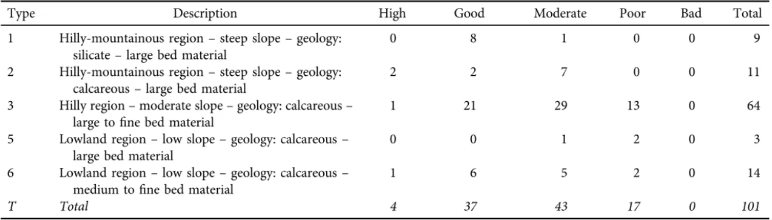
The river network of Hungary is subdivided into 1,078 water bodies, 889 of which are river water bodies, and the remaining ones are lake water bodies. This study was restricted to river water bodies whose long-term mean flow (LMQ) <1 m3s1. According to the 2nd River Basin Man- agement Plan of Hungary (GDWM 2015), the 889 river WBs are classified into types 1 to 10 based on their catch- ment size, relief, soil, and grain size characteristics (Table 3).
The studied water bodies belonged to types 1, 2, 3, 5, or 6 (WFD-CIS 2003). Most of them had the physico-chemical status of moderate or good, and none of them was bad (Table 3;Clement et al. 2015;Clement and Szilagyi 2015).
The watershed of each river was delineated based on EU- DEM v1.1 (Copernicus Land Monitoring Service 2016a) with the TauDEM method (Tarboton 1997;Fig. 2). EU-DEM also allowed for computing the basic relief properties of the wa- tersheds (Table 1). Land use shares were calculated on the basis of the Corine Land Cover 2012 database (Copernicus Land Monitoring Service 2016b). A cadaster of Hungarian waste- water treatment plants allowed for the calculation of point- source loads emitted to each river (GDWM 2016b). The emission values were divided by the long term mean flow (LMQ) of the river. The watershed properties served as pre- dictor variables in the discriminant analysis models.
Figure 2.Location of study sites. Thin black lines denote the study rivers; their watershed and location of monitoring sites are also indicated
Water quality data
The subject of the analyses was WQ data from 13 parameters (Table 2) available for 2007–2016 from Hungary, describing the salinity, acidity, oxygen budget, and nutrient conditions of the water bodies. Samples were gathered by one of the seven na- tional laboratories, and component concentrations were either measured on-site or in the laboratory, according to Hungarian
and international standards. The availability of WQ data restricted the number of creeks: only 101 of the total of 638
“small”(LMQ < 1 m3s1) rivers were involved in the study.
Methodology
A 13-element vector of WQ values characterized each water body according to the list of parameters (Table 2). The characteristic value of each parameter was the mean of all values measured at any location along the river. Parameter means were generated in two steps. First, a yearly mean value was calculated. Secondly, the mean of the yearly values was computed. This way, biases caused by eventual changes in sampling frequency (e.g. at different sites) could be eliminated. The values were then z-score transformed.
Listing all rivers (in alphabetical order) and parameters (in the above order) in a matrix formed our initial database (101313 matrix). This matrix determines the position of each river in the 13-dimensional space. The Euclidean dis- tance between each pair of points was then calculated and indicated in the distance matrix (DM): a square matrix of size 101. In the DM, small numbers indicate high similarity, while large ones indicate dissimilarities. By definition, the main diagonal of the DM consists of zeros indicating each water’s identity with itself. Instead of inserting the large matrix in this study, a novel but simple visualization tech- nique is used: values below a certain threshold are dimmed black, while the rest of the matrix is kept white.
In order to picture the magnitude of the transformed distance units, the above transformation was applied to distances between type 3 and type 6 class boundaries (Table 3). Distances between adjacent class boundaries vary between 4.2 and 6.1 (Table 4). This means that two WBs being two units distant from one another have a great Table 1.Properties of study water bodies and their watersheds. *high–1, good–2, moderate–3, poor–4, bad–5. LMQ5long term mean
flow in the river; TN5total nitrogen; TP5total phosphorus; WW5wastewater
Property Mean value Range (min–max) Units
Relief and hydrology
WS area 160 13–910 km2
Mean elevation 250 130–600 m a.s.l.
Mean slope 0.087 0.004–0.26 –
Mean slope of arable land 0.059 0.003–0.22 –
Long term mean precipitation 640 560–820 mm
LMQ at outflow point 0.27 0.026–0.96 m3s1
Land use
Share of urban land 0.079 0–0.48 –
Share of arable land 0.39 0–0.86 –
Share of forests and semi-natural areas 0.45 0.04–0.97 –
Share of wetlands and open water surfaces 0.0035 0–0.03 –
Point source loads
Total population 24,000 44–330000 –
WW discharge relative to LMQ 0.07 0–1.1 –
TN load from WW relative to LMQ 1.5 0–14 g m3
TP load from WW relative to LMQ 0.13 0–1.3 g m3
Result of status assessment
Status class* 2.72 1–4 –
Table 2.WQ parameters used in the study and their descriptive statistics for the selected WBs
Parameter Mean
Standard deviation
Measurement unit Acidity
PH 8.1 0.2 –
Salinity
Electric conductivity 940 400 mS cm1
Chloride ion concentration
54 46 g m3
Oxygen budget
Dissolved oxygen 8.8 3.9 g m3
Oxygen saturation 80 41 %
Biochemical oxygen demand
4.5 3.3 g m3
Chemical oxygen demand
22 12 g m3
Total organic carbon 8.4 4.1 g m3
Ammonium nitrogen 0.5 1.3 g m3
Nutrients Total inorganic
nitrogen
4.5 3.9 g m3
Total nitrogen 5.5 4.6 g m3
Orthophosphate 700 1100 g L1
Total phosphorus 410 480 g L1
chance to be ordered into the same status class. On the other hand, if the distance between them is six transformed units, then there is a very high probability for one of them being at least an entire class worse than the other. Following this, the thresholds for a value to be dimmed black was chosen to be either 2 (Fig. 3, left;Fig. 5) or 6 (Fig. 3, right).
Hierarchical Cluster Analysis (HCA)
Based on the DM, the hierarchical cluster dendrogram was generated (Day and Edelsbrunner 1984). During the clus- tering process, Ward’s minimum variance method (Ward 1963) was used to determine the distance between a new group and the previously created groups / nodes. The Ward’s method uses the analysis of variance approach to evaluate the distances between clusters while attempting to minimize the sum of squares of any two clusters that can be
formed at each step. Finally, the dendrogram was intersected so that three groups would be distinguished.
Linear Discriminant Analysis (LDA)
Linear discriminant analysis is a classification algorithm that uses predictor variables to find the function that mostly differentiates between a nominal categorical variable (dependent variable;McLachlan 1992;Duda et al. 2000). In the present study, LDA was used to attempt to reproduce the HCA groups (the dependent variable) using two sets of watershed properties as predictor variables. In two consec- utive models, the number of predictor variables was chosen to be 2 and 5 (Table 5).
Table 3.Occurrence of physico-chemical status classes in the unique water body types present in the study (GDWM 2015)
Type Description High Good Moderate Poor Bad Total
1 Hilly-mountainous region–steep slope–geology:
silicate–large bed material
0 8 1 0 0 9
2 Hilly-mountainous region–steep slope–geology:
calcareous–large bed material
2 2 7 0 0 11
3 Hilly region–moderate slope–geology: calcareous–
large tofine bed material 1 21 29 13 0 64
5 Lowland region–low slope–geology: calcareous– large bed material
0 0 1 2 0 3
6 Lowland region–low slope–geology: calcareous– medium tofine bed material
1 6 5 2 0 14
T Total 4 37 43 17 0 101
Table 4.Distance between class boundaries according to the metrics used in the study (type 3/type 6).
High/
good
Good/
moderate
Moderate/
poor
Poor/
bad
High/good 0 4.4 9.2 14
Good/moderate 5.6 0 6.0 12
Moderate/poor 8.7 4.2 0 6.1
Poor/bad 14 10 6.1 0
Figure 3.Distance matrix with WBs ordered alphabetically. Instead of indicating the unique numbers, a monochrome visualization tech- nique is used: small values are dimmed black while large values are white. Left and right matrices are identical, but the threshold for a value to be dimmed black is different: two on the left side and six on the right side
Table 5.Predictor variables in model 1 and model 2. WW5 wastewater.*Values indicate diffuse pollution, or its lack and, except for the slope, are meant relative to watershed area.**Values indicate point sources pollution values and area meant relative to
long term meanflow of the receiving water body.
Model 1 Model 2
Mean slope* þ
Share of arable land* þ þ
Share of forests* þ
WW discharge** þ
WW total nitrogen** þ
WW total phosphorus** þ
Calculations were performed in Microsoft Excel and R (packages stats and MASS; Venables and Ripley 2002; R Core Team 2019). This software, along with QGIS, was used to visualize results.
RESULTS
Distance analysis
The visualization technique described under Methodology allows for the identification of waters with extreme behavior: those being members of a tight group, or, the other extremity: being distant from (almost) all the others.
Black patches on Fig. 3 (left) indicate first-case waters.
These are small creeks with low or no human impact, sit- uated mostly in forested mountainous areas. Second-case waters are indicated by white horizontal and vertical lines onFig. 3(right); they are situated mostly in lowland urban or agricultural areas and thus disturbed by heavy human pollution.
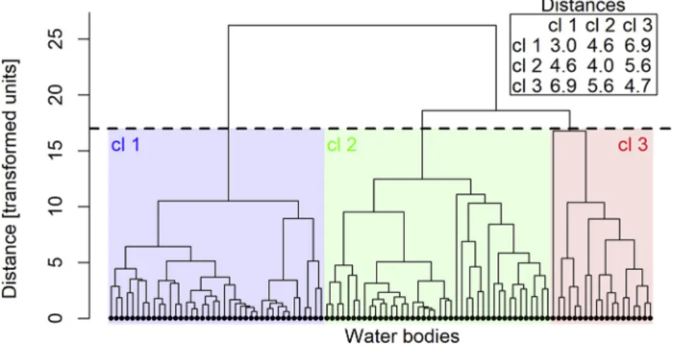
Grouping of water bodies
After grouping the water bodies with HCA based on the DM, a dendrogram was obtained (Fig. 4). The dendrogram was intersected at 70% of the maximum linkage distance, creating three clusters. It can be seen that not only are the members of Cluster 1 closer to each other than to any member of Clusters 2 or 3, but distances between members of Cluster 1 are smaller than those between members of Cluster 2 or Cluster 3. In order to visualize the tendency that mean intra-group distances increase from Cluster 1 to Cluster 3, previously alphabetically ordered elements of the DM were rearranged: members of Cluster 1 were gathered into the upper left corner, members of Cluster 2 stayed in the middle, and members of Cluster 3 got into the lower right corner. The density of black patches on this new figure (Fig. 5, left) also confirms the increasing ten- dency.
To link cluster grouping with river basin management plan (RBMP) classes, the DM was reordered again: this time according to the RBMP class of the WB (class bad was
Figure 4.Hierarchical clustering dendrogram. Dashed line: transection level.“cl 1”to“cl 3”: clusters 1 to 3 (also denoted by colors blue, green, and red). Table: Intra-group and inter-group mean distances
Figure 5.Distance matrix rearranged. Left: sorted according to clusters 1 to 3; right: sorted according to RBMP class. Instead of indicating the unique numbers, values <2 transformed units are dimmed black, and the rest are white. cl 35cluster 3; h5high
empty since no WB of the study fell into the worst class).
Mean intra-group distances were calculated for this grouping as well, resulting in values of 3.2, 3.1, 4.0, and 5.3 for classeshigh,good,moderate,and poor,respectively (see Fig. 5, right). When comparing the cluster group and the RBMP class for the unique WBs, it was found that 31 out of 40 WBs in Cluster 1 came from classeshighorgood, 29 out of 42 WBs in Cluster 2 came from classmoderateand 14 out of 19 WBs in Cluster 3 came from classpoor. Thisfinding demonstrates that the simple and straightforward method of hierarchical clustering was robust in reproducing the RBMP classes; or, the other way round: that RBMP class threshold values reflect the cluster boundaries quite well. Thisfinding serves as an additional verification of the class boundaries (Clement et al. 2015).
Prediction of grouping with LDA models
In Model 1, almost two-thirds of the WBs could be classified correctly into Clusters 1 to 3. In particular, 68, 69, and 26%
of WBs were correctly classified into Clusters 1, 2, and 3, respectively (Table 6). Since Model 1 only worked with two predictor variables, a two-dimensional visualization is possible (Fig. 6).
Model 2 allowed for a 12% increase in prediction accuracy compared to that of Model 1. The correctness rate increased for all three cluster groups (see the last column of Table 6).
Both models affirm that cluster groupings were in strong relationship with point-source and diffuse pollution loads.
DISCUSSION
Many previous studies documented the fact that land use, along with point-source loads, determines the clustering of monitoring sites (Wang et al. 2014; Zhou et al. 2016).
Zhou et al. (2016)even concluded that clusters are created according to the degree of human point-source and diffuse impacts. The novel visualization technique used in this study led to the conclusion that undisturbed WBs show higher clustering inclination than heavily polluted ones.
On the one hand, this is a direct consequence of the fact that the parameter set in this study was chosen to represent anthropogenic effects. Higher concentrations mean higher disturbance. On the other hand, this means that the quality of unpolluted water is much more predictable based on background properties than that of a highly polluted one.
In other words, pollution can take many, quite varied, forms.
The share of agricultural land along with other land uses being the most critical predictor variables of water quality is in good agreement with many previous studies (Chen et al. 2016 – agricultural land; Bu et al. (2014) – agricultural þbuilt-up; Mehaffey et al. (2005)– agricul- turalþ“developed”). Besides arable land, the main factors should be impervious/urban land along with forests, the latter having a positive effect on WQ, except for forest roads (Sliva and Williams 2001;Jaafari et al. 2015;Angyal
Table 6.Cluster group properties
Cluster
Number of WBs in cluster
Total number of WQ samples in cluster
Number of WQ samples per WB
Mean intra- group distance
Prediction accuracy of model 1 [%]
Prediction accuracy of model 2 [%]
1 40 3044 76 3.0 68 85
2 42 2867 68 4.0 69 74
3 19 1492 79 4.7 26 42
Total 101 7403 73 3.7 60 72
Figure 6.Classified and predicted cluster groups. Point colors: blue, green, red correspond to clusters 1, 2, and 3, respectively. Background colors: light blue, dark green, and rose correspond to prediction areas for clusters 1, 2 and 3, respectively
et al. 2016;Barclay et al. 2016). According to ourfindings, WBs with no or meager wastewater share and arable land below 30% will likely have a good or high status. On the contrary, those with a wastewater share around or above 40% will not achieve good status. Status of WBs with wastewater share between 5 and 40%, arable land share above 30% is uncertain. These numbers are in good accordance with thefindings ofK€andler et al. (2017), who concluded that settlement areas govern the chemical signature if their proportion of the land use is above 20%, arable land rules the WQ when its proportion is above 40%
and that forest proportions bigger than 70% lead to WQ with low concentrations of pollutants.
Effects on the planning of future monitoring activities
The results of HCA and LDA are to be used for optimizing monitoring activities. Our study established that the current number of measurements is not in proportion with the complexity of the pollution problem (Table 6). In particular, WBs falling in Cluster 3 need more measurements, which can be carried out at the expense of members of Cluster 1, the latter being more similar to one another.
When planning monitoring activities on previously un- monitored small watercourses, the following guidelines must be respected:
Relatively fewer measurements are needed on WBs where WW share < 10% and arable land share < 30% because they are very likely to achievegoodstatus.
More measurements are needed on waters where arable land share > 30% or 40% < WW share < 70%, to track the desired status improvement.
The focus should be on WBs where 10% < WW share <
40% and / or 30% < arable land share because their status will probably be close to thegood/moderateborder.
WBs with WW share > 70% are very rare and probably have verybadstatus.
Evaluation, perspectives
The methodology presented in this paper is capable of estimating water quality based on watershed properties.
Nevertheless, it should not be concluded that measurements can be neglected (the method relies firmly on measurement data) but rather that measurements should be focused on water bodies at risk (i.e., those characterized with high hu- man impact). On the other hand, pristine waters have“more to lose”; therefore, their monitoring is also important (e.g.
F€olster et al. 2014).
Further investigation is needed to determine the sensitivity of the results to the WQ parameters chosen. A possible development of the presented methodology could be the taking into account of the (hydrological) distance of a land use and point-source inlet from the monitoring site.
CONCLUSIONS
Hierarchical clustering analysis was used to group 101 water bodies into three main groups based on their normalized physico-chemical measurement data. It was found that (1) clusters emerged according to the level of pollution in the water body and that (2) water bodies with no or low dis- turbances show higher similarities (smaller distances) among them than those with high pollution. It has been established that current monitoring practice puts too much emphasis on undisturbed waters while it does not deal suf- ficiently with heavily polluted ones. Concerning unmoni- tored waters, future monitoring should focus on those with WW share between 10 and 40% and arable land share above 30%, because in their case, only monitoring can decide whether they will achievegoodstatus.
ACKNOWLEDGMENTS
The research reported in this paper was supported by the Higher Education Excellence Program of the Ministry of Human Capacities in the frame of the Water Sciences &
Disaster Prevention research area of the Budapest University of Technology and Economics (BME FIKP-VIZ).
REFERENCES
Angyal, Z., Sark€ozi, E., Gombas,A., & Kardos, L. (2016). Effects of land use on chemical water quality of three small streams in Budapest. Open Geosciences, 8, 133–142. https://doi.org/10.
1515/geo-2016-0012.
Azhar, S. C., Aris, A. Z., Yusoff, M. K., Ramli, M. F., & Juahir, H.
(2015). Classification of river water quality using multivariate analysis. Procedia Environmental Sciences, 30, 79–84. https://
doi.org/10.1016/j.proenv.2015.10.014.
Barclay, J. R., Tripp, H., Bellucci, C. J., Warner, G., & Helton, A. M.
(2016). Do waterbody classifications predict water quality?
Journal of Environmental Management,183, 1–12.https://doi.
org/10.1016/j.jenvman.2016.08.071.
Behmel, S., Damour, M., Ludwig, R., & Rodriguez, M. J. (2016).
Water quality monitoring strategies – a review and future perspectives.Science of the Total Environment,571, 1312–1329.
https://doi.org/10.1016/j.scitotenv.2016.06.235.
Borics, G., Lukacs, B. A., Grigorszky, I., Laszlo-Nagy, Z., G-Toth, L., Bolgovics, A., Szab o, S., G€orgenyi, J., & Varbıro, G. (2014).
Phytoplankton-based shallow lake types in the Carpathian ba- sin: steps towards a bottom-up typology. Fundamental and Applied Limnology, 184, 23–34. https://doi.org/10.1127/1863- 9135/2014/0518.
Bostanmaneshrad, F., Partani, S., Noori, R., Nachtnebel, H. P., Berndtsson, R., & Adamowski, J. F. (2018). Relationship be- tween water quality and macro-scale parameters (land use, erosion, geology, and population density) in the Siminehrood
River Basin.Science of the Total Environment,639, 1588–1600.
https://doi.org/10.1016/j.scitotenv.2018.05.244.
Bu, H., Meng, W., Zhang, Y., & Wan, J. (2014). Relationships be- tween land use patterns and water quality in the Taizi River basin, China.Ecological Indicators,41, 187–197.https://doi.org/
10.1016/j.ecolind.2014.02.003.
Chapman, D. V., Bradley, C., Gettel, G. M., Hatvani, I. G., Hein, T., Kovacs, J., Liska, I., Oliver, D. M., Tanos, P., Trasy, B., (2016).
Developments in water quality monitoring and management in large river catchments using the Danube River as an example.
Environmental Science and Policy,64, 141–154.https://doi.org/
10.1016/j.envsci.2016.06.015.
Chen, Q., Mei, K., Dahlgren, R. A., Wang, T., Gong, J., & Zhang, M.
(2016). Impacts of land use and population density on seasonal surface water quality using a modified geographically weighted regression. Science of the Total Environment, 572, 450–466.
https://doi.org/10.1016/j.scitotenv.2016.08.052.
Clement, A. & Buzas, K. (1999). Use of ambient water quality data to refine emission estimates in the Danube basin.Water Science and Technology,40, 35–42.
Clement, A. & Somlyody, L. (2011). Vızmin}oseg-szabalyozas (Water quality management). In: Somlyody, L. (Ed.), Mag- yarorszag Vızgazdalkodasa: Helyzetkepes Strategiai Feladatok (Water management in hungary: situation report and strategic tasks). Hungarian Academy of Sciences, Budapest, pp. 169–206 (in Hungarian).
Clement, A. & Szilagyi, F. (2015). Felszıni vıztestek fizikai kemiai allapotertekelesi rendszere (Physico-chemical status evaluation system of surface waters). In:Orszagos Vızgy}ujt}o-gazdalkodasi Terv 2015, A Duna-vızgy}ujt}o Magyarorszagi Resze; OVGT 6–2 Hatteranyag (National river basin management plan 2015, Hungarian part of the Danube river basin, OVGT 6–2 back- ground material).General Directorate of Water Management Hungary, Budapest, p.15 (in Hungarian).
Clement, A., Szilagyi, F., & Kardos, M. K. (2015). Felszıni vizek min}osıtese az €okologiat tamogato fizikai-kemiai jellemz}ok szerint – az allapotertekeles tanulsagai az intezkedesi pro- gramok tervezese szempontjabol (Classification of surface wa- ters according to ecology-supporting physico-chemical quality elements – lessons learned during status evaluation, with respect to design of management interventions). In: Szlavik, L.
(Ed.), Proceedings of the XXXIII National Meeting of the Hungarian Hydrological Society. Hungarian Hydrological So- ciety, Budapest, pp. 1–11 (in Hungarian).
Congress, U. S. (1972).Federal Water Pollution Control Act.–33 U.S.C § 1251 et seq., https://www.boem.gov/environment/
environmental-assessment/federal-water-pollution-control-act- 1972-or-clean-water-act.
Copernicus Land Monitoring Service (2016a). European Digital Elevation Model (EU-DEM), version 1.1.https://land.copernicus.
eu/imagery-in-situ/eu-dem/eu-dem-v1.1 (Accessed 6 January 2019).
Copernicus Land Monitoring Service (2016b). Corine Land Cover (CLC) 2012, version 18.https://land.copernicus.eu/pan-european/
corine-land-cover/clc-2012(Accessed 1 January 2018).
Day, H. E. W. & Edelsbrunner, H. (1984). Efficient algorithms for agglomerative hierarchical clustering.Journal of Classification, 1/1, 7–24.
Duda, R. O., Hart, P. E., & Stork, D. G. (2000).Pattern classifica- tion, 2nd ed. John Wiley & Sons, New York, p. 650.
Dworak, T., Gonzalez, C., Laaser, C., & Interwies, E. (2005). The need for new monitoring tools to implement the WFD.Envi- ronmental Science and Policy, 8, 301–306. https://doi.org/10.
1016/j.envsci.2005.03.007.
EEA. (2018).European waters–assessment of status and pressures.
European Ennvironment Agency, Luxembourg, p. 90, https://
doi.org/10.2800/303664.
F€olster, J., Johnson, R. K., Futter, M. N., & Wilander, A. (2014). The Swedish monitoring of surface waters: 50 years of adaptive monitoring. AMBIO, 43, 3–18. https://doi.org/10.1007/s13280- 014-0558-z.
GDWM. (2015). Vızfolyas es allovız tipologia. 1–2. szamu hatteranyag az Orszagos Vızgy}ujt}o-gazdalkodasi Tervek 2015.
evi fel€ulvizsgalatahoz (River and lake water typology. back- ground document no. 1–2 to the revision of the National River Basin Management Plans 2015). General Directorate of Water Management Hungary, Budapest, p. 9. (in Hungarian).
GDWM. (2016a).Felszıni vıztestek€okologiaies kemiaiallapota. 6–
1. szamu melleklet az Orszagos Vızgy}ujt}o-gazdalkodasi Tervek 2015.evi fel€ulvizsgalatahoz (Ecological and chemical status of surface waters. Supplement no. 6–1 to the National River Basin Management Plans 2015). General Directorate of Water Man- agement Hungary, Budapest (in Hungarian).
GDWM. (2016b).Szennyvızterheles jellemz}oi: kommunalises ipari szennyvızkibocsatas. 3–1 szamu melleklet az Orszagos Vızgy}ujt}o- gazdalkodasi Tervek 2015. evi fel€ulvizsgalatahoz (Wastewater load characteristics: urban and industrial effluent data. Sup- plement no. 3–1 to the National River Basin Management Plans 2015). General Directorate of Water Management Hungary, Budapest (in Hungarian).
Giri, S. & Qiu, Z. (2016). Understanding the relationship of land uses and water quality in twentyfirst century: a review.Journal of Environmental Management,173, 41–48.https://doi.org/10.
1016/j.jenvman.2016.02.029.
Giri, S., Qiu, Z., & Zhang, Z. (2018). Assessing the impacts of land use on downstream water quality using a hydrologically sen- sitive area concept.Journal of Environmental Management,213, 309–319.https://doi.org/10.1016/j.jenvman.2018.02.075.
Hatvani, I. G., Kovacs, J., Kovacs, I. S., Jakusch, P., & Korponai, J.
(2011). Analysis of long-term water quality changes in the Kis- Balaton Water Protection System with time series-, cluster analysis and Wilks’lambda distribution.Ecological Engineering, 37, 629–635.https://doi.org/10.1016/j.ecoleng.2010.12.028.
Hatvani, I. G., Clement, A., Kovacs, J., Kovacs, I. S., & Korponai, J.
(2014). Assessing water-quality data: The relationship between the water quality amelioration of Lake Balaton and the con- struction of its mitigation wetland. Journal of Great Lakes Research,40, 115–125.https://doi.org/10.1016/j.jglr.2013.12.010.
HSI. (1993). Felszıni vizek min}osege, min}osegi jellemz}okes min- }
osıtes, Magyar Szabvany 12749 (Quality of surface water, quality characteristics and classification, Hungarian National Standard Nr. 12749). Hungarian Standardization Institute, Budapest, p.
12. (in Hungarian).
Jaafari, A., Najafi, A., Rezaeian, J., & Sattarian, A. (2015). Modeling erosion and sediment delivery from unpaved roads in the north mountainous forest of Iran.GEM – International Journal on
Geomathematics, 6, 343–356. https://doi.org/10.1007/s13137- 014-0062-4.
Johnson, S. (2006).The Ghost Map. Riverhead Books, New York, p.
332.
K€andler, M., Blechinger, K., Seidler, C., Pavlu, V.,Sanda, M., Dostal, T., Krasa, J., Vitvar, T., &Stich, M. (2017). Impact of land use on water quality in the upper Nisa catchment in the Czech Republic and in Germany.Science of the Total Environment,586, 1316–
1325.https://doi.org/10.1016/j.scitotenv.2016.10.221.
Kerekes-Steindl, Z. (2016). Water quality protection in Hungary– policy and status.Hungarian Journal of Hydrology,96, 43–56.
Kovacs, J., Tanos, P., Korponai, J., Kovacs-Szekely, I., Gondar, K., Gondar-S}oregi, K., & Hatvani, I. G. (2012a). Analysis of water quality data for scientists. In: Voduris, K. & Voutsa, D. (Eds.), Water quality monitoring and assessment. IntechOpen, London, pp. 65–94.https://doi.org/10.5772/32173.
Kovacs, J., Nagy, M., Czauner, B., Kovacs, I. S., Borsodi, A. K., &
Hatvani, I. G. (2012b). Delimiting sub-areas in water bodies using multivariate data analysis on the example of Lake Balaton (W Hungary). Journal of Environmental Management, 110, 151–158.https://doi.org/10.1016/j.jenvman.2012.06.002.
Kovacs, J., Kovacs, S., Magyar, N., Tanos, P., Hatvani, I. G., & Anda, A.
(2014). Classification into homogeneous groups using combined cluster and discriminant analysis.Environmental Modelling and Software,57, 52–59.https://doi.org/10.1016/j.envsoft.2014.01.010.
Kovacs, J., Kovacs, S., Hatvani, I. G., Magyar, N., Tanos, P., Korponai, J., & Blaschke, A. P. (2015). Spatial optimization of monitoring networks on the examples of a river, a Lake-Wetland system and a Sub-Surface water system. Water Resources Management, 29, 5275–5294.https://doi.org/10.1007/s11269-015-1117-5.
Laszlo, B., Szilagyi, F., Szilagyi, E., Heltai, G., & Licsko, I. (2007).
Implementation of the EU Water Framework Directive in monitoring of small water bodies in Hungary, I. Establishment of surveillance monitoring system for physical and chemical characteristics for small mountain watercourses.Microchemical Journal,85, 65–71.
McLachlan, G. J. (1992). Discriminant analysis and statistical pattern recognition, 1st ed. John Wiley & Sons, New York, p.
526,https://doi.org/10.1002/0471725293.
Mehaffey, M. H., Nash, M. S., Wade, T. G., Ebert, D. W., Jones, K.
B., & Rager, A. (2005). Linking land cover and water quality in New York City’s water supply watersheds. Environmental Monitoring and Assessment, 107, 29–44. https://doi.org/10.
1007/s10661-005-2018-5.
Novotny, V. & Olem, H. (1994). Water quality – prevention, identification and management of diffuse pollution, 1st ed. van Nostrand Reinhold, New York, p. 1054.
R Core Team. (2019).R: a language and environment for statistical computing. R Foundation for Statistical Computing, https://
www.r-project.org/(Accessed 1 January 2019).
R€oman, E., Ekholm, P., Tattari, S., Koskiaho, J., & Kotam€aki, N.
(2018). Catchment characteristics predicting nitrogen and phosphorus losses in Finland.River Research and Applications, 34, 397–405.https://doi.org/10.1002/rra.3264.
Shimada, Y. (2018). A history of water quality monitoring system in Japan. In: Yoneda, M. & Mokhtar, M. (Eds.),Environmental risk analysis for Asian-oriented, risk-based watershed
management. Springer, Singapore, pp. 163–168.https://doi.org/
10.1007/978-981-10-8090-6_13.
Sliva, L. & Williams, D. D. (2001). Buffer zone versus whole catchment approaches to studying land use impact on river water quality.Water Research,35, 3462–3472.https://doi.org/
10.1016/S0043-1354(01)00062-8.
Somlyody, L. (2018).Felszıni Vizek Min}osege (surface water qual- ity). Typotex, Budapest, p. 372. (in Hungarian).
Strobl, R. O. & Robillard, P. D. (2008). Network design for water quality monitoring of surface freshwaters: a review.Journal of Environmental Management, 87, 639–648. https://doi.org/10.
1016/j.jenvman.2007.03.001.
Szabo, A. (2008).Hattervaltozok szerepe a Dunaes a Tisza€okologiai min}osıteseben (Role of background variables in ecological qual- ification of Danube and River Tisza). PhD Thesis, University of Debrecen, Debrecen, p. 124.
Tango, P. J. & Batiuk, R. A. (2016). Chesapeake Bay recovery and factors affecting trends: long-term monitoring, indicators, and insights. Regional Studies in Marine Science,4, 12–20.https://
doi.org/10.1016/j.rsma.2015.11.010.
Tanos, P., Kovacs, J., Szekely, I., & Hatvani, I. G. (2011). Explor- atory data analysis on the Upper-Tisza section using single and multi-variate data analysis methods.Central European Geology, 54, 345–356.https://doi.org/10.1556/CEuGeol.54.2011.4.3.
Tanos, P., Kovacs, J., Kovacs, S., Anda, A., & Hatvani, I. G. (2015).
Optimization of the monitoring network on the River Tisza (Central Europe, Hungary) using combined cluster and discriminant analysis, taking seasonality into account. Envi- ronmental Monitoring and Assessment,187/9, 1–14.https://doi.
org/10.1007/s10661-015-4777-y.
Tarboton, D. G. (1997). A new method for the determination of flow directions and upslope areas in grid digital elevation models.Water Resources Research,33, 309–319.
Telci, I. T., Nam, K., Guan, J., & Aral, M. M. (2009). Optimal water quality monitoring network design for river systems.Journal of Environmental Management,90, 2987–2998.https://doi.org/10.
1016/j.jenvman.2009.04.011.
Trasy, B., Garamhegyi, T., Laczko-Dobos, P., Kovacs, J., & Hatvani, I. G. (2018). Geostatistical screening of flood events in the groundwater levels of the diverted inner delta of the Danube River: implications for river bed clogging. Open Geosciences, https://doi.org/10.1515/geo-2018-0006.
Tsakiris, G. & Alexakis, D. (2012). Water quality models: an overview.European Water,37, 33–46.
Tu, J. & Xia, Z. G. (2008). Examining spatially varying relationships between land use and water quality using geographically weighted regression I: Model design and evaluation.Science of the Total Environment,407, 358–378.https://doi.org/10.1016/j.
scitotenv.2008.09.031.
Varbıro, G., Borics, G., Csanyi, B., Feher, G., Grigorszky, I., Kiss, K. T., Toth, A., & Acs, E. (2012). Improvement of the ecological water qualification system of rivers based on thefirst results of the Hungarian phytobenthos surveillance monitoring.
Hydrobiologia,695, 125–135.https://doi.org/10.1007/s10750-012- 1120-2.
Varol, M., G€okot, B., Bekleyen, A., & S¸en, B. (2012). Spatial and temporal variations in surface water quality of the dam
reservoirs in the Tigris River basin, Turkey.Catena,92, 11–21.
https://doi.org/10.1016/j.catena.2011.11.013.
Venables, W. N. & Ripley, B. D. (2002).Modern applied statistics with S-plus. Springer, New York, p. 495.
Wang, Y. Bin, Liu, C. W., Liao, P. Y., & Lee, J. J. (2014).
Spatial pattern assessment of river water quality: Implica- tions of reducing the number of monitoring stations and chemical parameters. Environmental Monitoring and Assessment, 186, 1781–1792. https://doi.org/10.1007/s10661- 013-3492-9.
Ward, J. H. (1963). Hierarchical grouping to optimize an objective function. Journal of the American Statistical Association, 58, 236–244.https://doi.org/10.1080/01621459.1963.10500845.
Wetzel, R. G. (2001).Limnology: lake and river ecosystems, 3rd ed.
Academic Press, San Diego, p. 1006.
WFD-CIS. (2003).Guidance document no 10: reference conditions, common implementation strategy for the WFD. Guidance Documents, European Comission, p. 274, https://doi.org/10.
2779/53333.
Wunderlin, A. D., Dıaz, M., Ame, M. V., Pesce, F. S., Hued, A. C., &
Bistoni, M. (2001). Pattern recognition techniques for the evaluation of spatial and temporal variations in water quality. A case study: Suquıa River basin (Cordoba-Argentina). Water Research, 35, 2881–2894. https://doi.org/10.1016/S0043- 1354(00)00592-3.
Zhou, P., Huang, J., Pontius, R. G., & Hong, H. (2016). New insight into the correlations between land use and water quality in a coastal watershed of China: Does point source pollution weaken it?Science of the Total Environment,543, 591–600.https://doi.
org/10.1016/j.scitotenv.2015.11.063.
Open Access statement.This is an open-access article distributed under the terms of the Creative Commons Attribution 4.0 International License (https://
creativecommons.org/licenses/by/4.0/), which permits unrestricted use, distribution, and reproduction in any medium, provided the original author and source are credited, a link to the CC License is provided, and changes–if any–are indicated. (SID_1)