The Descriptional Complexity of Rewriting Systems - Some Classical and Non-Classical Models

(1)

The Descriptional Complexity of Rewriting Systems - Some Classical and Non-Classical

Models

by

Gy¨orgy Vaszil

Doctoral dissertation presented to the Hungarian Academy of Sciences

2013.

(2)

(3)

Chapter 1 Introduction

In this chapter we give a brief overview of the topics presented in this dissertation. First we will introduce the models of computation we will study.

We start with the classical model of formal grammars and describe some of their regulated variants. Next we move on to the field of grammar systems dealing with networks of grammars which cooperate in jointly generating a language, and then we introduce the non-classical notion of membrane systems, a chemical type of computing model dealing with the transformations of multisets of objects. Finally we describe our understanding of the term descriptional complexity, a field of research which we will be dealing with in the rest of the chapters.

1.1 Formal grammars with regulation

First we deal with regulated grammars, that is, context-free grammars with some additional control mechanism to regulate the use of the rules during the derivations.

The need for rewriting devices which use rules of a simple form but still have a considerable generative power is justified by the study of phenomena occurring in different areas of mathematics, linguistics, or even developmental biology. To study problems in these areas which cannot be described by the capabilities of context-free languages, it is often desirable to construct generative mechanisms which have as many context-free-like properties as possible, but are also able to describe the non-context-free features of the specific problem in question. See (Dassow and P˘aun, 1989) for a discussion

(6)

about non-context-free phenomena in different areas, and also (Dassow et al., 1997a) for regulated rewriting in general.

Tree controlled grammarswere introduced in ( ˇCulik II and Maurer, 1977) as a pair (G, R) where G is a context-free grammar and R is a regular set, called the control language. The control language contains words composed of the terminal and nonterminal alphabets ofG, and it is used to control the work of G by restricting the set of derivations which G is allowed to make.

Only those words belong to the generated language of the tree controlled grammar which can be generated by the context-free grammar G, and moreover, which have a derivation tree where all the strings obtained by reading from left to right the symbols labeling nodes which belong to the same level of the tree (with the exception of the last level) are elements of the regular set R.

As it was already shown in ( ˇCulik II and Maurer, 1977), tree controlled grammars are able to generate any recursively enumerable language. Variants of the notion with control sets which are not regular but belong to different classes from the Chomsky hierarchy were studied in (P˘aun, 1979), the power of subregular control sets were examined in more detail in (Dassow et al., 2010).

We also consider a different way of using the sentential form to control the rule application. It is based on the presence/absence of certain symbols or substrings in the sentential forms. One variant of this general idea is realized by conditional grammars, sometimes also called grammars with regular restriction, see (Frˇıs, 1968), (Salomaa, 1973). The derivations in these mechanisms are controlled by regular languages associated to the context- free rules: A rule can only be applied to the sentential form if it belongs to the language associated to the given rule.

A weaker restriction is used in the generative mechanisms called semi-conditional grammars, see (Kelemen, 1984), (P˘aun, 1985). These are context- free grammars with a permitting and a forbidding condition associated to each production. The conditions are given in the form of two words: a permitting and a forbidding word. A production can only be used on a given sentential form if the permitting word is a subword of the sentential form and the forbidding word is not a subword of the sentential form. Note that semi- conditional grammars are special cases of conditional grammars, since the sets of those sentential forms which satisfy the conditions associated to the rules are regular sets. Semi-conditional grammars are also known to generate the class of recursively enumerable languages.

(7)

The study of semi-conditional grammars continued with the introduction of simple semi-conditional grammarsin (Meduna and Gopalaratnam, 1994).

We speak of a simple semi-conditional grammar if each rule has at most one nonempty condition, that is, no controlling context condition at all, or either a permitting, or a forbidding one. Simple semi-conditional grammars were introduced in (Meduna and Gopalaratnam, 1994) where they were also were shown to be able to generate all recursively enumerable languages.

Finally, we will study scattered context grammars. Scattered context grammars, introduced in (Greibach and Hopcroft, 1969), also represent a class of generative devices which use the presence/absence of certain symbols or substrings in their current sentential forms to achieve additional control over the application of their rewriting rules.

The productions of these grammars are ordered sequences of context-free rewriting rules which have to be applied in parallel on nonterminals appearing in the sentential form in the same order as the nonterminals on the left- hand sides of the rules appear in the production sequence. Scattered context grammars are known to characterize recursively enumerable languages, see (Gonczarowski and Warmuth, 1989), (Meduna, 1995b), (Meduna, 1995a), and (Virkkunen, 1973).

1.2 Parallel communicating grammar systems

Due to their theoretical and practical importance, computational models based on distributed problem solving systems have been in the focus of interest for a long time. A challenging area of research concerning these systems is to elaborate syntactic frameworks to describe the behavior of communities of communicating agents which cooperate in solving a common problem, where the framework is sufficiently sophisticated but relatively easy to handle. The theory of grammar systems ((Dassow et al., 1997b), (Csuhaj-Varj´u et al., 1994)) offers several constructs for this purpose. One of them is the parallel communicating (PC) grammar system (introduced in (P˘aun and Sˆantean, 1989)), a model for communities of cooperating problem solving agents which communicate with each other by dynamically emerging requests.

In these systems, several grammars perform rewriting steps on their own sentential forms in a synchronized manner until one or more query symbols, that is, special nonterminals corresponding to the components, are introduced in the strings. Then the rewriting process stops and one or more

(8)

communication steps are performed by substituting all occurrences of the query symbols with the current sentential forms of the component grammars corresponding to the given symbols. Two types of PC grammar systems are distinguished: In the case of returning systems, the queried component re- turns to its start symbol after the communication and begins to generate a new string. In non-returning systems the components continue the rewriting of their current sentential forms. The language defined by the system is the set of terminal words generated by a dedicated component grammar, the master. In this framework, the grammars represent problem solving agents, the nonterminals open problems to be solved, the query symbols correspond to questions addressed to the agents, and the generated language represents the problem solution. Non-returning systems describe the case when the agent after communication preserves the information obtained so far, while in the case of returning systems, the agent starts its work again from the beginning after communicating information. The reader may notice that the framework of PC grammar systems is also suitable for describing other types of distributed systems, for example, networks with information providing nodes.

The relationship between the class of languages generated by returning and non-returning PC grammar systems have long been an important open problem in the field of PC grammars. First in (Mihalache, 1994), non- returning centralized PC grammar systems were simulated by returning but non-centralized systems, then in (Dumitrescu, 1996) a simulation was presented also for the general non-centralized case.

The exact characterization of the generative power of PC grammar systems has been an open problem for about ten years, until in (Csuhaj-Varj´u and Vaszil, 1999) returning PC grammar systems were shown to characterize the class of recursively enumerable languages. At the same time, (Mandache, 2000) showed that all recursively enumerable languages can also be generated by non-returning systems, but the construction of the proof did not provide an upper bound for the number of component grammars.

Returning to the original motivation, namely, to the description of the behavior of communities of problem solving agents, several natural problems arise. One of them is to study systems where clusters or teams of agents represent themselves as separate units in the problem solving process. Notice that this question is also justified by the area of computer-supported team work or cluster computing. The idea of teams has already been introduced in the theory of grammar systems for so-called cooperating distributed (CD)

(9)

grammar systems and eco-grammar systems, with the meaning that a team is a collection of components which act simultaneously (see (Kari et al., 1995),(P˘aun and Rozenberg, 1994), (Mateescu et al., 9394), (ter Beek, 1996), (ter Beek, 1997), (Csuhaj-Varjú and Mitrana, 2000), (Lázár et al., 2009)).

Inspired by these considerations, in (Csuhaj-Varj´u et al., 2011) we introduced the notion of a parallel communicating grammar system with clusters of components (a clustered PC grammar system, in short) where instead of individual components, each query symbol refers to a set of components, a (predefined) cluster. Contrary to the original model where any addressee of the issued query is precisely identified, i.e., any query symbol refers to exactly one component, here a cluster is queried, and anyone of its components is allowed to reply. This means that the clusters of components behave as separate units, that is, the individual members of the clusters cannot be distinguished at the systems’ level.

1.3 Membrane systems

Membrane systems, or P systems were introduced in (P˘aun, 2000) as computing models inspired by the functioning of the living cell. Their main components are membrane structures consisting of membranes hierarchically embedded in the outermost skin membrane. Each membrane encloses a region containing a multiset of objects and possibly other membranes. Each region has an associated set of operators working on the objects contained by the region. These operators can be of different types, they can change the objects present in the regions or they can provide the possibility of trans- ferring the objects from one region to another one. The evolution of the objects inside the membrane structure from an initial configuration to a somehow specified end configuration correspond to a computation having a result which is derived from some properties of the specific end configuration. Several variants of the basic notion have been introduced and studied proving the power of the framework, see the monograph (P˘aun, 2002) for a comprehensive introduction, the recent handbook (P˘aun et al., 2010) for a summary of notions and results of the area, and (Ciobanu et al., 2006) for various applications.

One of the most interesting variants of the model was introduced in (P˘aun and P˘aun, 2002) called P systems with symport/antiport. In these systems the modification of the objects present in the regions is not possible, they

(10)

may only move through the membranes from one region to another. The movement is described by communication rules called symport/antiport rules associated to the regions. (This phenomenon also has analogues in biology, see (Alberts et al., 1994) for more details).

A symport rule specifies a multiset of objects that might travel through a given membrane in a given direction, an antiport rule specifies two multisets of objects which might simultaneously travel through a given membrane in the opposite directions. The result can be read as the number of objects present inside a previously given output membrane after the system reaches a halting configuration, that is, a configuration when no application of any rule in any region is possible.

Note the important role that the environment plays in the computations of membrane systems which use only communication rules: the type and number of objects inside the system can only be changed by sending out some of them into the environment, and importing some others from the environment. Thus, we need to make assumptions also about the environment in which the system is placed.

The situation is similar also in the case of P colonies, the other membrane system variant we will discuss. They represent a class of membrane systems similar to so-called colonies of simple formal grammars (Kelemen and Kele- menová, 1992) (see also (Csuhaj-Varjú et al., 1994; Dassow et al., 1997b) for basic elements of grammar systems and (Csuhaj-Varjú et al., 1997) for the Artificial Life inspired eco-grammar systems).

1.4 Descriptional complexity - A brief over- view of the following chapters

In this dissertation we understand the term descriptional complexity as an area of theoretical computer science studying various measures of complexity of grammars, automata, or related system (measuring the succintness of their descriptions) and the relationships, trade-offs, between the different variants of systems for a given measure, or the different variants of measures for a given system.

Descriptional complexity aspects of systems (automata, grammars, rewriting systems, etc.) have been a subject of intensive research since the beginning of computer science, but the field has also been actively studied in

(11)

recent years. Examples of some early results of the type we are interested in, appeared in (Gruska, 1969) about the size of context-free grammars, and the size measures of the number of nonterminal symbols and the number of productions were also introduced, see also (Kelemenov´a, 1982) for a survey of “grammatical complexity” of context-free grammars. The succintness of representations of languages by different variants of automata were also considered by several authors, see (Goldstine et al., 2002) and (Holzer and Kutrib, 2011) for more details, and a survey of results in these areas.

It is clear that the fact that a system is able to simulate some universal device implies that its size parameters can be bounded. This holds, since by simulating the universal device, all computations are carried out by a fixed (universal) system (having, therefore, fixed size parameters). On the other hand, it is still interesting to look for the best possible values of the bounds, or to study the relationship of certain size parameters with each other or with other properties of the given system.

In Chapter 3 we consider some variants of regulated grammars. Natu- ral measures of descriptional complexity for a formal grammar (regulated or not) are the number of nonterminal symbols and the number of productions (rewriting rules). In addition to measuring the complexity of the grammar, studying measures which also take into account the complexity of the control mechanism is also of interest. Concerning tree controlled grammars we will study the number of nonterminals of the underlying grammar plus the minmal number of nonterminals necessary to generate the control language which is used to regulate the derivations. In simple semi-conditional grammars, we investigate the number of productions and the size of the context conditions used for controlling the rule application. Finally, for scattered- context grammars, we consider the number of nonterminal symbols and the number of context sensing priductions.

In the Chapter 4 we deal with networks of cooperating grammars and focus our attention on parallel communicating grammar systems. These are systems of cooperating context-free grammars, so instead of the complexity of the individual components, we would like to focus our attention on the complexity of the system as described by its size, that is, the number of components, and the complexity of the cooperation, that is, the communication protocol. Concerning the types of communication, we first describe the relationship of the returning or non-returning variants, then we reduce the complexity of the communication in the network by showing how to group some of the individual components into clusters which are, in some sense,

(12)

indistinguishable at the systems’ level.

In Chapter 5 we first investigate some descriptional complexity aspects of symport/antiport P systems. We consider symport/antiport rules with minimal cooperation, that is, symport rules moving just one object and antiport rules moving two objects, one in each direction. (These are in some sense the “smallest” possible rules of this type.) We examine the number of membranes necessary for systems having these simple rules to reach the maximal power, that is, to generate recursively enumerable sets. In the second part of the chapter we consider P colonies. First we show how to bound the number of cells, the number of programs, or both of these measures simultaneously.

Then we further simplify the already very simple components of these systems by introducing insertion/deletion programs in such a way that some cells are only able to export objects into the environment, while others are only able to consume objects from the environment. Finally we restrict the number of objects inside the cells of the P colony and study systems which have only one object, the minimal possible amount, inside the cells.

(13)

Chapter 2 Some Preliminary Definitions and Notation

In this chapter we present some general definitions and notation which will be used in the subsequent parts of the text. The reader is assumed to be familiar with the basic notions of formal languages and automata theory, more details can be found in the handbook (Rozenberg and Salomaa, 1997), or the monographs (Salomaa, 1973) and (Dassow and P˘aun, 1989).

2.1 Generative grammars

A finite set of symbols T is called an alphabet. The cardinality, that is, the number of elements ofT is denoted by |T|. The set of non-empty words over the alphabetT is denoted byT⁺; the empty word isε, andT^∗ =T⁺∪ {ε}.A setL⊆T^∗is called a language overt.For a wordw∈T^∗ and a set of symbols A ⊆T, we denote the length ofw by |w|, and the number of occurrences of symbols from A in w by |w|A. If A is a singleton set, i.e., A = {a}, then we write |w|_a instead of |w|_{a}. The concatenation of two sets L1, L2 ⊆ V^∗, denoted as L₁L₂, is defined as L₁L₂ ={w₁w₂ |w₁ ∈L₁, w₂ ∈L₂}.

A generative grammar G is a quadruple G = (N, T, S, P) where N and T are the disjoint sets of nonterminal and terminal symbols, S ∈ N is the initial nonterminal, and P is a set of rewriting rules (or productions) of the form α → β where α, β ∈ (N ∪ T)^∗ with |α|N ≥ 1. A string v can be derived from a string u, denoted as u⇒v for some u, v ∈(N ∪T)^∗, if they can be written as u = u₁αu₂, v = v₁βv₂ for a rewriting rule α → β ∈ P.

(14)

The reflexive and transitive closure of the relation ⇒is denoted by⇒^∗. The language generated by the grammarGis the set of terminal strings which can be derived from the initial nonterminal, that is, L(G) = {w∈T^∗ |S ⇒^∗ w}.

It is known that any recursively enumerable language can be generated by a generative grammar defined as above.

A generative grammar is context-free, if the rewriting rules α → β are such, that α ∈ N. A context-free grammar is regular, if in addition to the property that α ∈ N, it also holds, that β ∈ T^∗ ∪ T^∗N. The classes of recursively enumerable, context-free, and regular grammars and languages are denoted by RE, CF, REG, L(RE), L(CF), and L(REG), respectively.

2.2 Counter machines

An n-counter machine M = (T ∪ {Z, B}, E, R, q₀, q_F), n ≥ 1, is an n+ 1- tape Turing machine where T is an alphabet, E is a set of internal states with two distinct elements q0, qF ∈E, andR is a set oftransition rules. The machine has a read-only input tape and n semi-infinite storage tapes (the counters). The alphabet of the storage tapes contains only two symbols, Z and B (blank), while the alphabet of the input tape isT ∪ {B}. The symbol Z is written on the first, leftmost cells of the storage tapes which are scanned initially by the storage tape heads, and may never appear on any other cell.

An integer t can be stored by moving a tape headt cells to the right ofZ. A stored number can be incremented or decremented by moving the tape head right or left. The machine is capable of checking whether a stored value is zero or not by looking at the symbol scanned by the storage tape heads. If the scanned symbol is Z, then the value stored in the corresponding counter is zero (which cannot be decremented since the tape head cannot be moved to the left ofZ). We will sometimes refer to the number stored in the counter as the contents of the counter, and we will call a counter empty when the stored number is zero.

The rule set R contains transition rules of the form (q, x, c1, . . . , cn) → (q^′, e1, . . . , en) where x∈ T ∪ {B} ∪ {ε} corresponds to the symbol scanned on the input tape in state q ∈ E, and c1, . . . , cn ∈ {Z, B} correspond to the symbols scanned on the storage tapes. By a rule of the above form, M enters state q^′ ∈E, and the counters are modified according to e1, . . . , en ∈ {−1,0,+1}. If x ∈ T ∪ {B}, then the machine scanned x on the input tape, and the head moves one cell to the right; if x = ε, then the machine

(15)

performs the transition irrespectively of the scanned input symbol, and the reading head does not move.

A configuration of then-counter machineM can be denoted by a (n+ 2)- tuple (w, q, j1, . . . , jn) where w ∈ T^∗ is the unread part of the input word written on the input tape, q ∈ Q is the state of the machine, and ji ∈ N, 1 ≤ i ≤ n, is the value stored on the ith counter tape of M. For two configurations, C and C^′, we write C ⊢a C^′ if M is capable of changing the configuration C = (aw, q, j1, . . . , jn) to C^′ = (w, q^′, j₁^′, . . . , j_n^′) by reading a symbol a ∈ T ∪ {ε} from the input tape and applying one of its transition rules.

A word w ∈ T^∗ is accepted by the machine if starting in the initial configuration (w, q0,0, . . . ,0), the input head eventually reaches and reads the rightmost non-blank symbol on the input tape, andM is in the accepting state qF, that is, it reaches a configuration (ε, qF, j1, . . . , jn) for some ji ∈ N, 1≤i≤n. The language accepted by M is denoted by L(M).

It is known that 2-counter machines (written from now on astwo-counter machines) are computationally complete; they are able to recognize any re- cursively enumerable language (see (Fischer, 1966)). Obviously, n-counter machines for any n >2 are of the same accepting power.

We will also use a variant of the above notion from (Minsky, 1967), the notion of a register machine. It consists of a given number of registers each of which can hold an arbitrarily large non-negative integer number (we say that the register is empty if it holds the value zero), and a set of labeled instructions which specify how the numbers stored in registers can be ma- nipulated.

Formally, a register machine is a construct M = (m, H, l0, lh, R), where m is the number of registers, H is the set of instruction labels, l0 is the start label, lh is the halting label, andR is the set of instructions; each label from H labels only one instruction fromR. There are several types of instructions which can be used. For li, lj, lk ∈H and r∈ {1, . . . , m} we have

• li : (nADD(r), lj, lk) -nondeterministic add: Add 1 to registerrand then go to one of the instructions with labels lj or lk, nondeterministically chosen.

• li : (ADD(r), lj) - deterministic add: Add 1 to register r and then go to the instruction with label lj.

• li : (SUB(r), lj) - subtract: If register r is non-empty, then subtract one

(16)

from it, otherwise leave it unchanged, and go to the instruction with label lj in both cases.

• li : (CHECK(r), lj, lk) -zero check: If the value of register r is zero, go to instruction lj, otherwise go to lk.

• lh :HALT - halt: Stop the machine.

A register machine M computes a set N(M) of numbers in the following way: It starts with empty registers by executing the instruction with label l0

and proceeds by applying instructions as indicated by the labels (and made possible by the contents of the registers). If the halt instruction is reached, then the number stored at that time in register 1 is said to be computed by M. Because of the nondeterminism in choosing the continuation of the computation in the case of nADDinstructions, N(M) can be an infinite set.

Note that register machines can be defined without thenADDinstructions as deterministic computing devices which compute some function of an input value placed initially in an input register. It is known (see, e.g., (Minsky, 1967)) that in this way they can compute all functions which are Turing computable. We added the nondeterministic add instruction in order to obtain a device which generates sets of numbers starting from a unique initial configuration. As any recursively enumerable set can be obtained as the range of a Turing computable function on the set of non-negative integers, this way we can generate any recursively enumerable set of numbers.

2.3 Multisets

We end this chapter by presenting the necessary notions and notions necessary for the use of multisets. A multiset over an arbitrary (not neces- sarily finite) set V is a mapping M : V → N which assigns to each object a ∈ V its multiplicity M(a) in M. The support of M is the set supp(M) = {a | M(a) ≥ 1}. If V is a finite set, then M is called a finite multiset. The set of all finite multisets over the finite set V is denoted by V^∗. We say that a ∈ M if M(a) ≥ 1, the cardinality of M, card(M) is defined as card(M) = T_a∈MM(a). For two multisets M₁, M₂ : V → N, M1 ⊆M2 holds, if for all a ∈V, M1(a) ≤M2(a). The union of M1 and M2

is defined as (M1 ∪M2) : V → N with (M1 ∪M2)(a) = M1(a) +M2(a) for alla∈V, the difference is defined forM₂ ⊆M₁ as (M₁−M₂) :V →N with

(17)

(M1−M2)(a) =M1(a)−M2(a) for all a ∈V. A multiset M is empty if its support is empty, supp(M) =∅.

We will represent a finite multiset M over V by a string w over the alphabetV with|w|a =M(a), a∈V, andεwill represent the empty multiset.

(18)

Chapter 3 Grammars with Regulation

In this chapter we present results about computational models studied in the area of regulated rewriting. These models are constructed by adding some kind of a control mechanism to ordinary (usually context-free) grammars which restricts the application of the rules in such a way that some of the derivations which are possible in the usual derivation process are eliminated from the controlled variant. This means that the set of words generated by the controlled device is a subset of the original (context-free) language generated without the control mechanism. As these generated subsets can be non-context-free languages, these mechanisms are usually more powerful than ordinary (context-free) grammars. See (Dassow and P˘aun, 1989) for more details, and also (Dassow et al., 1997a) for regulated rewriting in general.

Since it has been always important to describe formal languages as con- cisely and economically as possible, it is of interest to study these mechanisms from the point of view of descriptional complexity. As the measures of complexity of the descriptions, we will study the number of nonterminals, the number of production rules, and the complexity of the added control mechanism.

3.1 Preliminaries

In the next sections we will use normal form results from (Geffert, 1988) stating that all recursively enumerable languages can be generated by grammars in which there are only a few rules which are not context-free (linear context-free, to be more precise). The idea of the normal forms is based on

(19)

the fact that for each L∈ L(RE) there are two homomorphismsh1, h2, such that w∈ L, if and only if there is an α with h1(α) =h2(α)w. (This can be shown similarly to the undecidability of the so called Post correspondence problem.) Based on the above homomorphisms, one can construct a grammar which generates words of the form wβ1β2 where β1 = h(h1(α)) and β2

is the reverse of h(h2(α)w) for some encoding h, and then generates w by deleting β1β2 if and only if they are mirror images of each other.

These ideas were converted into normal form results by (Geffert, 1988) as follows. If L ⊆ T^∗ is a recursively enumerable language, then L can be generated by a grammar

G= (N, T, P ∪ {AB →ε, CD →ε}, S),

such that N ={S, S^′, A, B, C, D}, andP contains only context-free productions. Furthermore, the context-free rules of G are of the form

S →zSx, where z ∈ {A, C}^∗, x∈T, S →S^′,

S^′ →uS^′v, where u∈ {A, C}^∗, v ∈ {B, D}^∗, S^′ →ε.

Considering the rules above, we can distinguish three phases in the generation of a terminal word x₁. . . x_n, x_i ∈T,1≤i≤n.

1. S ⇒^∗ zn. . . z1Sx1. . . xn⇒zn. . . z1S^′x1. . . xn, where zi ∈ {A, C}^∗,1≤i≤n.

2. zn. . . z1S^′x1. . . xn ⇒^∗ zn. . . z1um. . . u1S^′v1. . . vmx1. . . xn ⇒ zn. . . z1um. . . u1v1. . . vmx1. . . xn,

where uj ∈ {A, C}^∗, vj ∈ {B, D}^∗,1 ≤ j ≤ m. Now the terminal string x1. . . xn is generated by G if and only if, using AB → ε and CD → ε the substring zn. . . z1um. . . u1v1. . . vm can be erased

3. zn. . . z1um. . . u1v1. . . vmx1. . . xn⇒^∗ x1. . . xn.

This can be successful if and only if zn. . . z1um. . . u1 = g(v1. . . vm)^R where g :{B, D} → {A, C} is a morphism with g(B) = A and g(D) =C.

We will refer to the three stages of a derivation of a grammar in the normal form above as the first, the second, and thethird phase.

(20)

It is not difficult to see that if we encode the nonterminal A to XY, the nonterminalB toZ, the nonterminalC toX, and the nonterminalDtoY Z, then one erasing rule of the form XY Z → ε is sufficient to have the same effect as AB →ε and CD →ε together.

Thus, all recursively enumerable languages L⊆ T^∗ can be generated by a grammar

G= (N, T, P ∪ {ABC →ε}, S),

such thatN ={S, S^′, A, B, C}, andP contains only context-free productions of the form

S→zSx, where z ∈ {A, B}^∗, x∈T, S→S^′,

S^′ →uS^′v, where u∈ {A, B}^∗, v ∈ {B, C}^∗, S^′ →ε.

The three phases of the derivation can also be distinguished in this case. In order to successfully generated a terminal word x1. . . xn, xi ∈ T,1≤ i ≤ n, first we need to generate a sentential form with the terminal prefix x1. . . xn, then continue with the generation of the nonterminal suffix (these are the first two phases), and finally (in the third phase) we need to erase all the nonterminals.

Notice that the nonterminal S^′ and the ruleS →S^′ can be eliminated in both normal form variants above. The three derivational phases cannot be

“mixed” in any successful derivation even if only S is used instead ofS and S^′.

The number of nonterminals of a generative grammar G = (N, T, S, P) is denoted by Var(G), that is, Var(G) = |N|. For a language L and a class of grammars X ∈ {REG,CF}, we denote by Var_X(L) the minimal number of nonterminals necessary to generate Lwith a grammar of type X, that is, VarX(L) = min{Var(G)|L=L(G) and G is of type X ∈ {REG,CF}}.

3.2 Tree controlled grammars - The number of nonterminals and the complexity of the control langauge

Investigations concerning the nonterminal complexity of tree controlled grammars began in (Turaev et al., 2011b) where this measure was defined as the

(21)

sum of the number of nonterminals of the context-free grammar and the number of nonterminals which are necessary to generate the regular control language. They showed that nine nonterminals altogether are sufficient to generate any recursively enumerable language with a tree controlled grammar. Then this bound was improved to seven in (Turaev et al., 2011a) by simulating a phrase structure grammar being in the Geffert normal form (see the second variant presented in Section 3.1 without the distinguished S and S^′), that is, having four nonterminals and only linear context-free productions, together with one non-context-free production in addition which is able to erase three neighboring nonterminals as it is of the form ABC →ε.

In this section we show how to improve the bound from seven to six using a similar technique as in (Turaev et al., 2011a), but simulating a grammar being in a different version of the Geffert normal form (see the first variant presented in Section 3.1): Instead of the non-context-free productionABC → ε, it has two non-context-free productions AB → ε, CD → ε. Since the nonterminals, A, B, C, D, will be encoded in the simulating tree controlled grammar by strings over just two symbols, it does not matter that instead of the symbols A, B, C we need to simulate a grammar which uses more symbols, A, B, C, D. On the other hand, the fact that instead of three, only two neighboring symbols have to be deleted simultaneously, helps to construct a simulating tree controlled grammar which uses one nonterminal less than the one in (Turaev et al., 2011a), thus helps to reduce the bound on the number of necessary nonterminals from seven to six.

For the introduction of tree controlled grammars, we need the notion of the derivation tree. An ordered tree is a derivation tree of a context- free grammar G = (N, T, S, P) if its nodes are labeled with symbols from N∪T∪ {ε} in a way which satisfies the following properties: (a) The root is labeled with S, (b) the leaves are labeled with symbols fromT∪ {ε}, and (c) every interior vertex is labeled from N in such a way that if a vertex has a labelA ∈N and its children are labeled from left to right withx1, x2, . . . , xm, xi ∈ N ∪T ∪ {ε}, 1 ≤ i ≤ m, then there is a production A → x1x2. . . xm

in P. A derivation tree corresponds to a terminal word w from L(G) if the concatenation of the symbols labeling the leaves of the tree from left to right coincide with w.

The distance of a vertext from the root is the length of the shortest path leading to t from the root node. The string corresponding to the ith level of a derivation tree for some i ≥ 0 is the word obtained by concatenating from left to right the symbols labeling those nodes of the tree which are at

(22)

distance ifrom the root.

Definition 3.2.1. A tree controlled grammar is a pair G = (G^′, R) where G^′ = (N, T, S, P) is a context-free grammar andR is a regular language over the alphabet N ∪T. The language L(G) generated by the tree controlled grammar G contains all words w ∈ T^∗ from L(G^′) which have a derivation tree where the strings corresponding to each different level, except the last one, belong to the regular set R.

The nonterminal complexity of a tree controlled grammar G = (G^′, R) is the number of nonterminals of G^′ plus the minimal number of nonterminals that a regular grammar needs for generating the language R, that is, Var(G) = Var(G^′) + VarREG(R).

To illustrate the notion of tree controlled grammars, let us recall an example from (Dassow and P˘aun, 1989).

Example 3.2.1. Let G= (G^′, R) where G^′ = ({S},{a}, S, P)with P ={S →SS, S →a} and R={S}^∗.

As the control language R contains words which are sequences of the non- terminal symbol S, all the nodes of every level (except the last one) of the derivation tree of a word w∈L(G) are labeled by the symbol S. This means that all the nonterminals, with the exception of the ones labeling the nodes directly above the last level of the tree, are rewritten by the rule S → SS, and the nonterminals of the level directly above the last one are rewritten by S →a. Thus, the language generated by G isL(G) ={a²ⁿ |n ≥0}.

We will also need the notion of unique-sum sets which was introduced in (Frisco, 2009) as follows. A set of nonnegative integers U = {u1, . . . , up} having the sum σU = Σ^p_i=1ui is said to be a unique-sum set, if the equation Σ^p_i=1ciui =σU forci ∈Nhas the only solutionci = 1, 1≤i≤p. Examples of unique-sum sets are {2,3}, {4,6,7}, or {8,12,14,15}, while the set {4,5,6}

is not unique-sum, as 4 + 5 + 6 = 15 = 5 + 5 + 5. It is clear that any subset of a unique-sum set is unique-sum, and that the sum of any two numbers from the set, σi,j =ui+uj, cannot be produced as the linear combination of elements of the set in any other way.

(23)

3.2.1 The number of nonterminals

Now we show that every recursively enumerable language can be generated by a tree controlled grammar with six nonterminals.

Theorem 3.2.1. For any recursively enumerable languageL, there exists a tree controlled grammar G with L=L(G), such that Var(G) = 6.

Proof. Let L ⊆ T^∗ be a recursively enumerable language generated by the Geffert normal form grammar G1 = ({S, A, B, C, D}, T, S, P) where T = {a₁, a2, . . . , at} and P = {AB → ε, CD → ε, S → ε} ∪ {S → ziSai, S → u_jSv_j |z_i, u_j ∈ {A, C}^∗, v_j ∈ {B, D}^∗,1≤i≤t,1≤j ≤s}.

Let us define the morphism h:{A, B, C, D}^∗ → {0,$}^∗ by h(A) = $0⁶$, h(B) = $0¹⁰$, h(C) = $0¹²$, h(D) = $0¹³$ which encodes four of the nonterminals of the grammar G1 as strings over two symbols. Notice that the length of the coding sequences forms the unique-sum set {8,12,14,15}.

Let us now construct the tree controlled grammar G = (G^′, R) where G^′ = (N, T, S, P^′) withN ={S, S^′,$,0,#},

P^′ = {S →h(z)Sa|S →zSa∈P, a∈T, z∈ {A, C}^∗} ∪ {S →S^′} ∪

{S^′ →h(u)S^′h(v)|S →uSv ∈P, u∈ {A, C}^∗, v ∈ {B, D}^∗} ∪ {S^′ →ε,$→$,$→#,0→0,0→#,#→ε},

and

R = ({S, S^′} ∪T ∪X1∪X2)^∗{#²⁰,#²⁹, ε}, where

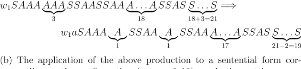
X1 = {$0⁶$,$0¹⁰$,$0¹²$,$0¹³$}, (3.1) X2 = {$0⁶$,$0¹⁰$}{#²⁰,#²⁹}{$0¹²$,$0¹³$}. (3.2) First we show that any terminal derivation ofG1 can be simulated by the tree controlled grammar G, that is, L(G₁)⊆L(G). Let w∈L(G₁) and let

S ⇒^∗ zSw⇒^∗ zuSvw ⇒zuvw (3.3)

be the first and the second phases of a derivation of w in G1 where z, u ∈ {A, C}^∗, v ∈ {B, D}^∗. We can generate h(zuv)w, the encoded version of zuvw with the rules of Gas follows

S ⇒^∗ h(z)Sw ⇒h(z)S^′w⇒^∗ h(zu)S^′h(v)w⇒h(zuv)w, (3.4)

(24)

h(zu) ∈ {$0⁶$,$0¹²$}^∗, h(v) ∈ {$0¹⁰$,$0¹³$}^∗. If we use the chain rules,

$ → $ and 0 → 0, we can make sure that the word corresponding to each level of the derivation tree belongs to the regular set R, and moreover, that h(zuv) is the string corresponding to the last level of the derivation tree which belongs to the derivation (3.4) of G above simulating the first two phases of the derivation of the word w in G1 depicted at (3.3).

Nowwcan be derived inG1 ifzuv can be erased by using the rulesAB → ε and CD→ε. IfAB orCD is a substring of zuv, then h(AB) = $0⁶$$0¹⁰$ or h(CD) = $0¹²$$0¹³$ is a substring of h(zuv), thus, one of the derivations

h(zuv)⇒h(zu^′)#²⁰h(v^′)w⇒h(zu^′v^′)w, or

h(zuv)⇒h(zu^′)#²⁹h(v^′)w⇒h(zu^′v^′)w

can be executed in G using the chain rules as above, and the rules 0 →

#, $ → #, # → ε in such a way that h(zu^′v^′) is again the string which corresponds to the last level of the derivation tree of h(zu^′v^′)w.

It is clear, that wheneverzuv can be erased inG₁, thenh(zuv) can also be erased inG, thus, wcan also be generated byGwhich means thatw∈L(G).

Now we show that L(G) ⊆ L(G1). To see this, we have to show that any w ∈ L(G) can also be generated by G1. Consider the derivation tree corresponding to a derivation of w ∈ L(G) in G and look at the words corresponding to the different levels of the tree.

Notice the following: (A) There is no symbol # appearing in the levels as long asS orS^′ is present. This statement holds because the words inRhave a special form: They are the concatenations of “complete” coding sequences of A, B, C, or D, that is, each subword over {$,0}is a concatenation of coding strings of the form $0ⁱ$ (for some i ∈ {6,10,12,13}). Thus, if # symbols appear in a word corresponding to a level of the derivation tree, then either all symbols of such a coding subword are rewritten to #, or no symbol of such a coding subword is rewritten to #. Recall that the lengths of these coding sequences form a unique-sum set, {8,12,14,15}, thus, 20 and 29 can only arise through some linear combination of the elements as 20 = 8 + 12, and 29 = 14 + 15. This, together with the above considerations, means that

#²⁰ or #²⁹ can only be obtained by rewriting all symbols of $0⁶$$0¹⁰$ or

$0¹²$$0¹³$ to #. Notice that when S or S^′ is present, then no sequence over {$0⁶$,$0¹²$}can be followed directly by a sequence over {$0¹⁰$,$0¹³$}, thus, when S orS^′ is present no neighboring code sequences of length 20 or

(25)

29 can occur which means that the words cannot contain #²⁰ or #²⁹ as a subsequence.

Statement (A) above implies that as long asSorS^′ is present in the words corresponding to the levels of the derivation tree, the chain rules $→$ and 0→0 have to be used on the symbols $,0 when passing to the next level of the derivation tree. This is also true for the word corresponding to the first level in which S^′ disappears after using a rule of the form S^′ → h(u)h(v), since uv 6= ε. Note that the part of the derivations of G with the presence of S and the presence ofS^′ corresponds to the first and the second phases of the derivations of the Geffert normal form grammar G1, respectively.

Consider now the first such level of the derivation tree corresponding to a derivation of winGin which none of the symbols S orS^′ are present. From the above considerations it follows that the string corresponding to this level has the formh(zu)h(v) whereh(zu)∈ {$0⁶$,$0¹²$}^∗,h(v)∈ {$0¹⁰$,$0¹³$}^∗, and zuvw can also be derived in the grammar G₁.

Note also: (B) There cannot be two distinct subsequences of the symbols

# in any of the words corresponding to any level of the derivation tree of the word w∈ L(G). To see this, consider the first level of the tree which is withoutSandS^′, and denote the string corresponding to this level ash(zuv).

Recall that h(zuv) = α1α2 where α1 ∈ {$0⁶$,$0¹²$}^∗, α2 ∈ {$0¹⁰$,$0¹³$}^∗, so subwords of the form {$0⁶$,$0¹²$}^∗{#²⁰,#²⁹}{$0¹⁰$,$0¹³$}^∗ can only be present in the words corresponding to subsequent levels of the tree in such a way that the sequence of # symbols is the result of rewriting a suffix of α1

and a prefix of α2 to #.

Property (B) above implies that in order to be in the control set R, a word which corresponds to some level of the derivation tree and also contains

#, must be of the form {$0⁶$,$0¹²$}^∗{#²⁰,#²⁹}{$0¹⁰$,$0¹³$}^∗ where #²⁰ or #²⁹ is obtained from the word corresponding to the previous level of the tree by rewriting each symbol in a substring $0⁶$$0¹⁰$ or $0¹²$$0¹³$ to

#, respectively. Therefore, the word corresponding to the previous level of the tree is either α₁^′$0⁶$$0¹⁰$α^′₂ or α^′₁$0¹²$$0¹³$α^′₂ where α₁^′ and α₂^′ satisfy either h⁻¹(α^′₁)AB h⁻¹(α₂^′) = zuv or h⁻¹(α^′₁)CD h⁻¹(α^′₂) = zuv provided that α1α2 =h(zuv).

This means that the uncoded version of the word corresponding to the next level of the derivation tree, where the # symbols are erased, can also be derived in G1 by the rules AB →ε orCD →ε. More precisely, the word corresponding to the next level of the derivation tree is either of the form α₁^′α^′₂ or α^′′₁{#²⁰,#²⁹}α^′′₂, all of them corresponding to the sentential form

(26)

h⁻¹(α^′₁)h⁻¹(α₂^′)w which can also be derived in G1.

Continuing the above reasoning, we obtain that the word corresponding to the level which is above the last one in the derivation tree of w∈L(G) is of the form #²⁰ or #²⁹, corresponding to the sentential form ABw or CDw in G1, thus, if w can be generated by the tree controlled grammar G with the control set R, then w can also be generated by the Geffert normal form grammar G1.

This means thatL(G)⊆L(G1), and since we have already shown the that the opposite inclusion holds, we haveL(G) =L(G1). As the control setRcan be generated by the regular grammar G2 = ({A}, T ∪ {0,$,#, S, S^′}, A, P2) with P2 ={A →xA, A→#²⁰, A→#²⁹, A→ε|x∈ {S, S^′} ∪T ∪X1 ∪X2

where X1 and X2 is defined as above at (3.1) and (3.2), respectively, and this grammar has just one nonterminal, we have proved the statement of the theorem.

3.2.2 Remarks

We have shown how to reduce the nonterminal complexity of tree controlled grammars from seven to six. This result first appeared in (Vaszil, 2012). We have used a similar technique as was used in (Turaev et al., 2011a), namely, we have simulated phrase structure grammars in the Geffert normal. There are two important differences, however, which have made it possible to realize the simulation with six nonterminals which number is one less than needed in (Turaev et al., 2011a) which contains the previously known best result.

First, instead of the normal form with the single erasing rule ABC →ε, we have used the variant with two erasing rules AB → ε, CD → ε, thus we needed to simulate the simultaneous erasing of only two nonterminals, as opposed to the simultaneous erasing of the three symbols in ABC →ε. The increase of the number of nonterminals (fromA, B, C toA, B, C, D) does not show up in the nonterminal complexity of the simulating grammar, since the nonterminal symbols are coded as words over two nonterminals.

The second modification concerns the way of coding the four nonterminals. We have used code words with lengths which form a unique-sum set.

This made the decoding possible with one less nonterminal than in (Turaev et al., 2011a).

Other language classes were also examined from the point of view of nonterminal complexity with respect to tree controlled grammars in (Turaev et al., 2012). Regular, linear, and regular simple matrix languages are shown

(27)

to be generated with three nonterminals which is an optimal bound, since there are regular languages which cannot be generated with two nonterminals. For context-free languages, on the other hand, four nonterminals are sufficient, although it is not known whether this bound cannot be decreased to three or not. In this paper it was also proved that any recursively enumerable language can be generated by a tree controlled grammar with seven nonterminals, but at the time of writing this dissertation, the result presented in the previous section is still the best result concerning the nonterminal complexity of tree controlled grammars generating recursively enumerable languages.

3.3 Simple semi-conditional grammars - The number of conditional productions and the length of the context conditions

In the case of semi-conditional grammars, the complexity of productions is measured by their degree, defined as the maximal length of the context conditions as a pair of integers, (i, j), where i and j is the length of the longest permitting and the longest forbidding word, respectively. In (P˘aun, 1985), recursively enumerable languages were characterized by semi-conditional grammars of degree (2,1) or (1,2), while grammars of degree (1,1) without erasing productions were shown to generate only a subclass of context-sensitive languages. The investigation of the generative power of grammars having only permitting or only forbidding conditions were also started, the language classes generated by grammars of degree (1,0) or (0,1) without erasing productions were shown to be strictly included in the class of context-sensitive languages.

In simple semi-conditional grammars, each rule has at most one nonempty condition, that is, no controlling context condition at all, or either a permitting, or a forbidding one. In (Meduna and Gopalaratnam, 1994), simple semi-conditional grammars of degree (1,2) and (2,1) were shown to be able to generate all recursively enumerable languages, but the number of rules necessary to obtain this power was unbounded.

The study of the number of productions necessary to obtain all recursively enumerable languages has been started in (Meduna and ˇSvec, 2002) where the authors prove that the class of recursively enumerable languages can be characterized by simple semi-conditional grammars of degree (2,1) with only

(28)

twelve conditional productions.

In this section we show how to improve the above mentioned bounds. We prove that ten conditional productions are sufficient to generate all recursively enumerable languages with grammars of degree (2,1), or eight of them are sufficient to generate all recursively enumerable languages with grammars of degree (3,1).

Definition 3.3.1. Asemi-conditional grammaris a constructG= (N, T, P, S) with nonterminal alphabet N, terminal alphabet T, a start symbol S ∈ N, and a set of productions of the form (X →α, u, v) withX ∈N,α∈(N∪T)^∗, and u, v ∈ (N ∪T)⁺∪ {0} where 0 6∈(N ∪T) is a special symbol. If either u6= 0 or v 6= 0, then the production is said to be conditional.

A semi-conditional grammar G has degree (i, j) if for all productions (X →α, u, v), u6= 0 implies |u| ≤i, and v 6= 0 implies |v| ≤j.

We speak of a simple semi-conditional grammar if each production has at most one nonempty condition, that is, if G = (N, T, P, S) is a simple semi-conditional grammar, then (X →α, u, v)∈P implies 0 ∈ {u, v}.

We say thatx∈(N∪T)⁺ directly derives y∈(N∪T)^∗ according to the rule (X → α, u, v) ∈ P, denoted by x ⇒ y, if x = x₁Xx₂, y = x₁αx₂ for some x1, x2 ∈(N∪T)^∗, and furthermore, u6= 0 implies thatu∈sub(x) and v 6= 0 implies that v 6∈sub(x).

If we denote the reflexive and transitive closure of ⇒ by ⇒^∗, then the language generated by a semi-conditional grammar G is L(G) = {w ∈ T^∗ | S ⇒^∗ w}.

Now let us recall an example from (Meduna and Gopalaratnam, 1994).

Example 3.3.1. Let G= ({S, A, X, C, Y},{a, b, c}, P, S) be a simple semi- conditional grammar with

P = {(S →AC,0,0), A→aXb, Y,0),(C →Y, A,0),(Y →Cc,0, A), (A→ab, Y,0),(Y →c,0, A),(X →A, C,0)}.

Note that Gis a simple semi-conditional grammar of degree(1,1), having six conditional productions.

Derivations of G start with

S ⇒AC ⇒ AY.

(29)

Assume that a string of the form a^kAb^kY c^k, k ≥ 0, can be generated by G.

We show that either a^k+1Ab^k+1Y c^k+1 or a^k+1b^k+1c^k+1 is generated by G, or the derivation is blocked.

The context conditions only allow the use of one of the rules A → aXb or A→ab. If the first one is chosen, then

a^kAb^kY c^k⇒a^k+1Xb^k+1Y c^k

is obtained and then one of the rules Y → c or Y → Cc must be used. If Y → c is chosen, the derivation can not continue because X can only be rewritten in the presence of a symbol C, so we must have

a^k+1Xb^k+1Y c^k⇒a^k+1Xb^k+1Cc^k+1 ⇒a^k+1Ab^k+1Cc^k+1 ⇒a^k+1Ab^k+1Y c^k+1. If having a^kAb^kY c^k we use the rule A→ab, we obtain

a^kAb^kY c^k ⇒a^k+1b^k+1Y c^k,

and the rule Y → Cc can not be used since C can only be rewritten in the presence of an A. So we must have

a^k+1b^k+1Y c^k⇒a^k+1b^k+1c^k+1.

From these considerations we can see that G generates the non-context-free language L(G) ={aⁿbⁿcⁿ|n ≥1}.

3.3.1 The number of conditional productions

In (Meduna and ˇSvec, 2002) the authors show that an erasing rule of the form XY → ε (X and Y being two nonterminals) can be simulated by six conditional productions of a simple semi-conditional grammar, thus, to simulate a grammar in the Geffert normal form (see the first variant presented in Section 3.1), simple semi-conditional grammars of degree (2,1) with twelve conditional productions are sufficient.

Now we show that any grammar being in the second variant of the Geffert normal form, thus, having only one non-context-free rule of the formABC → ε, (see Section 3.1), can be simulated by simple semi-conditional grammars of degree (2,1) with ten conditional productions.

Theorem 3.3.1. Every recursively enumerable language can be generated by a simple semi-conditional grammar of degree (2,1)having ten conditional productions.

(30)

Proof. Let L ⊆ T^∗ be a recursively enumerable language generated by the grammar

G= (N, T, P ∪ {ABC →ε}, S) as above.

Now we constructG^′, a simple semi-conditional grammar of degree (2,1) as follows. Let

G^′ = (N^′, T, P^′, S)

where N^′ ={S, S^′, A, A^′, B, B^′, B^′′, C, C^′, L, L^′, R}, and P^′ = {(X →α,0,0)|X →α∈P}

∪ {(A →LA^′,0, L),(B →B^′,0, B^′),(C →C^′R,0, R), (A^′ → ε, A^′B^′,0),(C^′ →ε, B^′C^′,0),(B^′ →B^′′, LB^′,0), (B^′′ →ε, B^′′R,0),(L→L^′, LR,0),(R →ε,0, L), (L^′ →ε,0, R)}.

By observing the productions of P^′, we can see that the terminal words generated by G can also be generated by the simple semi-conditional grammar G^′. In the following, we show that G^′ cannot generate words that are not generated by G.

We will examine the possible derivations of G^′ starting withS and leading to a terminal word. The first two phases of a derivation by G can be reproduced using the non-conditional rules of P^′, the rules of the form (X →α,0,0) where X →α ∈P. Since the conditional rules do not involve the symbols S and S^′ neither on the left or right sides, nor in the conditions, if we can apply conditional rules before S and S^′ both disappeared, then we can apply them in the same way also afterwards. According to this observa- tion, we can assume that the first application of a conditional rule happens when neither S, nor S^′ is present in the sentential form, that is, when the generated word is of the form

zuvw, where z, u∈ {A, B}^∗, v ∈ {B, C}^∗, w ∈T^∗.

Now we show that the prefix zuv can be deleted by the conditional rules of G^′ if and only if it can be deleted by the rule ABC →ε of G.

By continuing the derivation, at most one application of each of the rules (A → LA^′,0, L), (B → B^′,0, B^′), or (C → C^′R,0, R) can follow. If these rules do not produce any of the subwordsA^′B^′ orB^′C^′, the derivation cannot

The Descriptional Complexity of Rewriting Systems - Some Classical and Non-Classical Models