A Relational Database Model for Science Mapping Analysis
Manuel J. Cobo
Dept. Computer Science, University of Cádiz, Avda. Ramón Puyol s/n 11202 Algeciras, Cádiz, Spain. E-mail: manueljesus.cobo@uca.es
A. G. López-Herrera, Enrique Herrera-Viedma
Dept. Computer Science and Artificial Intelligence, University of Granada, C/Periodista Daniel Saucedo Aranda, s/n, E-18071 Granada, Spain. E-mail: lopez- herrera@decsai.ugr.es, viedma@decsai.ugr.es
Abstract: This paper presents a relational database model for science mapping analysis. It has been specially conceived for use in almost all of the stages of a science mapping workflow (excluding the data acquisition and pre-processing stages). The database model is developed as an entity-relations diagram using information that is typically presented in science mapping studies. Finally, several SQL queries are presented for validation purposes.
Keywords: Science Mapping Analysis; Bibliometric mapping; Bibliometric Studies;
Bibliometric networks; Co-word; Co-citation; Database model
1 Introduction
Online web-based bibliographical databases, such as ISI Web of Science, Scopus, CiteSeer, Google Scholar or NLM’s MEDLINE (among others) are common sources of data for bibliometric research [24]. Many of these databases have serious problems and usage limitations since they were mainly designed for other purposes such as information retrieval, rather than for bibliometric analysis [17].
In order to overcome these limitations, one common solution consists of downloading data from online databases, cleaning it and storing it in customized ad hoc databases [22]. However, it is difficult to find information on how these customized databases are designed or constructed.
The primary procedures in bibliometrics are science mapping analysis and performance analysis. Specifically, science or bibliometric mapping is an important research topic in the field of bibliometrics [23]. It is a spatial representation of how disciplines, fields, specialties and individual documents or authors are related with each other [31]. It focuses on the monitoring of a scientific field and the delimitation of a research area in order to determine its cognitive structure and evolution [7, 11, 19, 21, 25, 26]. In other words, science mapping is aimed at displaying the structural and dynamic aspects of scientific research [4, 23].
In order to analyze the dynamic and complex aspects of scientific activities, in science mapping research, the analyst needs methods of adequately managing the many-to-many relations between data elements (publications, authors, citations, and other variables) over time. The many-to-many relationship has been a recurrent problem in science mapping [8, 9].
Although a number of software tools have been specifically developed to perform a science mapping analysis [9], to our knowledge, there have been no proposals for efficient data modelling in a science mapping context. While some research has been published on basic bibliometrics databases [20, 32], a great deal of work still needs to be done on acceptable method for managing the special needs for data used in science mapping research [15].
Thus, this paper presents the first database model for science mapping analysis.
This database model has been specifically conceived for almost all of the stages of the classical science mapping workflow [9] – except for the stages of data acquisition and pre-processing. The database model is developed as an entity- relations diagram using information that is typically presented in science mapping studies [9].
This paper is structured as follows: In Section 2, the relational database model for science mapping analysis is presented. Section 3 offers a proof-of-concept for the relational database model, presenting several SQL and PL/SQL statements and procedures. Section 4 provides a practical example based on the proposed database model. Finally, some conclusions are drawn.
2 The Relational Database Model
Science mapping analysis is a bibliometric technique that allows for the uncovering of the conceptual, social and intellectual aspects of a research field.
Furthermore, the longitudinal framework allows us to highlight the evolution of these aspects across time. By combining science mapping analysis with bibliometric indicators [8], the analyst can detect the main topics of a research field, its hot topics and those that have had a greater impact (number of citations)
and have been the most productive. As described in [8], the science mapping analysis may be divided in the following steps:
1) To determine the substructures contained (primarily, clusters of authors, words or references) in the research field by means of a bibliometric network [5, 18, 27, 30] (bibliographic coupling, journal bibliographic coupling, author bibliographic coupling, co-author, co-citation, author co-citation, journal co- citation or co-word analysis) for each studied period.
2) To distribute the results from the first step in a low dimensional space (clusters).
3) To analyze the evolution of the detected clusters based on the different periods studied, in order to detect the main general evolution areas of the research field, their origins and their inter-relations.
4) To carry out a performance analysis of the different periods, clusters and evolution areas, based on bibliometric measures.
Thus, in this section we propose a database model for the science mapping analysis. The database model presented here has been specifically designed to work with co-occurrence networks, building the map through a clustering algorithm, and categorizing the clusters in a strategic diagram. Furthermore, it allows us to perform an evolution analysis in order to reveal the dynamical aspects of the analyzed field.
The database model has been designed to store all the information needed to begin the analysis, to perform the different steps of the methodology proposed in [8] and to maintain the obtained results.
Although the model does not visualize the results (graphically), these results may be easily exported using simple SQL queries in order to visualize them via visualization software such as Pajek [2], Gephi [3], UCINET or Cytoscape [29].
Subsequently, we shall discuss the raw data requirements and we shall analyze the conceptual design of the database model.
2.1 Requirements
The main aim of science mapping analysis is to extract knowledge from a set of raw bibliographic data. Usually, the analyst has previously downloaded the data from a bibliographic source and subsequently, imported it to a specific data model.
For example, the analyst could create a new spread sheet or load the data into a specific database.
Science mapping analysis uses several types of information: baseline or input data, intermediate data and results. The database model for science mapping analysis must be capable of storing these different types of information.
The baseline or input data is normally a set of documents with their set of associated units of analysis (author, references or terms). With this data, the analyst can build a bibliometric network. If the science mapping analysis is performed in a longitudinal framework, the documents should have an associated publication date.
It should be pointed out that the baseline data, especially the units of analysis, must have been pre-processed. In other words, the units of analysis need to have been previously cleaned, any errors should have been fixed, and the de-duplicating process must have been carried out previously. The data and network reduction is carried out using the database model as shown in Section 3.
As for intermediate data, the database model must be able to store a set of datasets (one per analyzed time slice or time period). Each dataset must have an associated set of documents, a set of units of analysis, the relationship between the documents and units, and finally, an undirected graph that represents the bibliometric network. In addition, the database model must be capable of generating intermediate data from the baseline data.
In regard to the resulting data, the database model must be capable of storing one set of clusters per dataset and an evolution map [8]. Also, a clustering algorithm is necessary in order to generate the map; however, since implementing this algorithm via SQL-queries could be a daunting task, it may be implemented using PL/SQL procedures.
Each cluster could have an associated set of network measures, such as Callon’s centrality and density measure [6]. Furthermore, each node of a bibliometric network, or even each cluster, may have an associated set of documents, and they could be used to conduct a performance analysis [8]. For example, we may calculate the amount of documents associated with a node, the citations achieved by those documents, the h-index, etc.
Finally, regarding the functionality requirements, the database model should be capable of the following:
- Building a set of datasets from the baseline data.
- Filtering the items of the datasets based on a frequency threshold.
- Extracting a co-occurrence network.
- Filtering the edges of the network using a co-occurrence threshold.
- Normalizing the co-occurrence network based on different similarity measures.
- Extracting a set of clusters per dataset.
- Adding different network measures to each detected cluster.
- Adding a set of documents to each detected cluster.
- Building an evolution map using the clusters of consecutive time periods.
2.2 Conceptual Design: the EER Diagram
In this section, we describe the database model, showing the different entities and relations that are necessary to develop a complete science mapping analysis. The Enhanced Entity/Relations (EER) data modeling is used to design the database in a conceptual way [14]. Thus, the EER diagram for the proposed database is shown in Figure 1.
We should point out certain notations that are used in the EER diagram. Each entity is represented as a box and the lines between two boxes represent a relationship between them. The cardinality of a relationship is represented as a number over the line. Each box has a title, which describes the entity’s name.
Thus, the proposed database model consists of five blocks: Knowledge Base, Dataset, Bibliometric Network, Cluster and Longitudinal. Each block is represented by a different color-shadow in Figure 1. These blocks are described below.
The Knowledge Base block is responsible for storing the baseline data. In order to conduct the science mapping analysis with the database model presented in this paper, the analyst should provide these entities filled out, or at least, offer the baseline data ready to be inserted in the corresponding entities, typically using insert-into SQL statements.
As mentioned previously, in order to perform a science mapping analysis under a longitudinal framework, the baseline data must consist, at least, of four entities:
Document, Publish Date, Period and Unit of Analysis. In order to fit with different kind and format of baseline date, we should point out that the proposed structure for this block may differ in some aspects from the implementation carried out by the analyst. In that case, only the queries to fill the dataset (Query 1 to 3) should be adapted to the particular structure.
The main entity of the Knowledge Base block is Document, which represents a scientific document. This entity stores the primary information, such as the title, abstract or citations received. This is the minimum information to identify a scientific document, and therefore, the analyst may expand upon this entity in order to add more information.
The Knowledge Base block contains two related pieces of longitudinal information: Publish Date, and Period. The former represents the specific date or year when the document was published. A Document must have one associated Publish Date, and a Publish Date has an associated set of Documents. The latter represents a slice of time or a period of years. The entity Period shall be used to divide the documents into different subsets in order to analyze the conceptual, social or intellectual evolution (depending on the kind of unit of analysis used).
Figure 1 EER diagram
Although the periods are usually disjoint set of years, we should point out that they may not necessarily be disjoint, so a year could appear in various periods.
Therefore, a Period consists of a set of Publish Dates, and a Publish Date can belong to one or more Periods.
The Unit represents any type of units of analysis that may be associated with a document, usually, the authors, terms or references. Our database model allows for the storage of only one type of unit of analysis at the same time. Regardless, it
shall be easy to replicate the analysis using other types of units. Since the documents usually contain a set of authors, terms and references, there is a many- to-many relationship between the Document and Unit entities.
When the science mapping analysis is carried out under a longitudinal framework, all of the data must be split into different slices which are usually referred to as periods. Each slice must contain a subset of documents and its related units of analysis, and therefore, the frequency of the units of analysis may differ for each slice.
Therefore, the Dataset block contains the entities that are responsible for storing a slice of the overall data. The Dataset block contains three entities: i) the Dataset, ii) the Documents of the dataset (DatasetDocument in Figure 1) and iii) the Unit of the dataset (DatasetUnit in Figure 1).
The Dataset is the main entity of this block. Since the remaining entities are related to a specific dataset, it is necessary during the followings steps. The Dataset is associated with a specific Period and it contains attributes such as a name to describe the slice, different parameters to filter the dataset and the network, and finally, the configuration of the clustering algorithm.
Each dataset consists of a set of documents and units of analysis. The documents are a subset of documents belonging to a specific period and the units are the subset of units associated with these documents. Since the units should be filtered using a minimum frequency threshold, each unit contains a Boolean attribute to indicate if it was filtered or not. Like the many-to-many relationship between the entities Document and Unit, there is a many-to-many relationship between the Documents of the dataset and the Units of the dataset (represented by the entity DatasetItem). It should also be noted that the same document-unit relationship may appear in different datasets.
The Bibliometric Network block consists of only one entity (NetworkPair) which stores the co-occurrence network of each dataset. Conceptually, this entity stores the network pairs. Each pair consists of a source node and a target node, with each node being a unit of a specific dataset. Each pair contains a weight (usually the co- occurrence count of both nodes in the dataset) and a normalized weight. As in Units, each pair may be filtered using a minimum co-occurrence threshold, thus there is a Boolean attribute to indicate if the pair has been filtered or not.
It is important to note that because the co-occurrence network is an undirected graph, the adjacency network representing the bibliometric network is a symmetric matrix. In other words, the source-target pair, and target-source pair should have the same weights and therefore, the same normalized weights.
The Cluster block contains four entities in order to represent the cluster itself and its properties. The Cluster entity belongs to a specific dataset, so there is a one-to- many relationship between the Dataset and Cluster entities. Furthermore, a Cluster is associated with a set of units of analysis. Moreover, the Cluster contains an
optional attribute that represents the main node of the cluster, usually the most central node of the associated sub-network [8].
As described in [9], a network analysis and a performance analysis could be applied to a set of clusters. Thus, the database model should be capable of storing the results of both analyses.
Although the results of the performance analysis are usually numerical measures (number of documents, sum of citations, average citations per document, h-index, etc.), they are calculated with a set of documents. Therefore, since each cluster contains a set of nodes (units of analysis) and each node is associated with a set of documents, the set of documents may be associated with each cluster using a document mapper function [10].
Thus, each cluster may contain two types of properties: i) measures and ii) a set of documents. As for the possible measures, network measures (Callon’s centrality and density measure), or performance measures (citations received by the documents associated with the cluster, and the h-index) may be defined as cluster properties.
Finally, the Longitudinal block stores the results of the temporal or longitudinal analysis. Specifically, it contains an entity to represent an Evolution map [8].
The evolution map can be defined as a bipartite graph showing the evolving relationship between the clusters of two consecutive periods [8]. Therefore, the Evolution map entity consists of a cluster source and a cluster target (each one belonging to different datasets) and a weight (evolution nexus) to represent the similarity between the source and target clusters.
3 Proof of Concept
This section shows how to develop a science mapping analysis using the database model presented in this paper. To accomplish this, we propose using different SQL-queries in order to perform the different steps of the analysis, proving that a science mapping analysis may in fact be conducted based on our database model.
As previously mentioned, the general workflow of a science mapping analysis includes a sequence of steps: data retrieval, data pre-processing, network extraction, network normalization, mapping, analysis, visualization and interpretation. Furthermore, each science mapping software tool [9] customizes or redefines its own workflow based on the general steps.
Thus, in order to develop a science mapping analysis using the database model presented in this paper, the analyst must follow a particular workflow analysis. It is important to note that, as mentioned in Section 2.1, both the data acquisition and data pre-processing tasks must have been carried out previously. That is, the
science mapping analysis workflow described in this section begins with pre- processed data.
The workflow analysis may be divided into four stages:
1) Building the dataset.
2) Extracting the bibliometric network.
3) Applying a clustering algorithm.
4) Carrying out network, performance and longitudinal analyses.
The first stage includes building the dataset from the data stored in the Knowledge Base block. For this, the documents, units and their relationships must be divided into distinct subsets, corresponding to each period. The different data- slices must be inserted in the corresponding entities, and associated with a specific dataset. The first stage is divided into five steps:
1) To insert the different datasets and associate them with a period. This step may be carried out using INSERT-INTO SQL statements. Since it is dependent upon the nature of the data, we have not included the queries for this step.
2) To extract the units of analysis for each dataset (Query 1).
3) To extract the documents for each dataset (Query 2).
4) To extract the relationships between documents and units of each dataset (Query 3).
5) To filter the units using the frequency threshold specified for each dataset (Query 4).
INSERT INTO DatasetUnit (DatasetUnit_idDataset, DatasetUnit_idUnit, DatasetUnit_frequency) SELECT p.Period_idPeriod, u.Unit_idUnit, count(u.Unit_idUnit)
FROM Period p, PublishDate_Period pup, PublishDate pu, Document d, Document_Unit du, Unit u WHERE
p.Period_idPeriod = pup.PublishDate_Period_idPeriod AND
pup.PublishDate_Period_idPublishDate = pu.PublishDate_idPublishDate AND pu.PublishDate_idPublishDate = d.Document_idPublishDate AND d.Document_idDocument = du.Document_Unit_idDocument AND du.Document_Unit_idUnit = u.Unit_idUnit
GROUP BY p.Period_idPeriod, u.Unit_idUnit;
Query 1
Retrieving the units of analysis for each dataset
INSERT INTO DatasetDocument (DatasetDocument_idDataset, DatasetDocument_idDocument) SELECT p.Period_idPeriod, d.Document_idDocument
FROM Period p, PublishDate_Period pup, PublishDate pu, Document d WHERE
p.Period_idPeriod = pup.PublishDate_Period_idPeriod AND
pup.PublishDate_Period_idPublishDate = pu.PublishDate_idPublishDate AND pu.PublishDate_idPublishDate = d.Document_idPublishDate;
Query 2
Retrieving the documents for each dataset
INSERT INTO DatasetItem (DatasetItem_idDataset, DatasetItem_idDocument, DatasetItem_idUnit) SELECT p.Period_idPeriod, d.Document_idDocument, du.Document_Unit_idUnit
FROM Period p, PublishDate_Period pup, PublishDate pu, Document d, Document_Unit du WHERE
p.Period_idPeriod = pup.PublishDate_Period_idPeriod AND
pup.PublishDate_Period_idPublishDate = pu.PublishDate_idPublishDate AND pu.PublishDate_idPublishDate = d.Document_idPublishDate AND d.Document_idDocument = du.Document_Unit_idDocument;
Query 3
Adding the relationships between documents and units (items) of analysis
UPDATE DatasetUnit SET DatasetUnit_isFiltered = 1
WHERE DatasetUnit_frequency < (SELECT d.Dataset_minFrequency FROM Dataset d
WHERE d.Dataset_idDataset = DatasetUnit_idDataset);
Query 4 Filtering the units of analysis
The second stage consists of extracting the bibliometric network for each dataset using the co-occurrence relation between the units of analysis. Then, the co- occurrence relations must be filtered and normalized. This stage is divided into three steps:
1) Building the bibliometric network by searching the co-occurrence relationships (Query 5).
2) Filtering the bibliometric network (pairs) using the specific co-occurrence threshold defined by each dataset. (Query 6).
3) Normalizing the bibliometric network using a similarity measure [13], such as, Salton's Cosine, Jaccard's Index, Equivalence Index, or Association Strength.
Query 7 shows the general query to carry out the normalization of a bibliometric network. In order to apply a specific similarity measure, the analyst must replace the text “SIMILARITY-MEASURE” in Query 7 with one of the formulas shown in Query 8.
INSERT INTO NetworkPair (NetworkPair_idDataset, NetworkPair_idNodeA, NetworkPair_idNodeB, NetworkPair_weight) SELECT d.DatasetDocument_idDataSet, di1.DatasetItem_idUnit AS nodeA, di2.DatasetItem_idUnit AS nodeB,
count(DISTINCT d.DatasetDocument_idDocument) AS coOccurrence
FROM DatasetDocument d, DatasetItem di1, DatasetUnit du1, DatasetItem di2, DatasetUnit du2 WHERE
d.DatasetDocument_idDataSet = di1.DatasetItem_idDataset AND d.DatasetDocument_idDocument = di1.DatasetItem_idDocument AND di1.DatasetItem_idDataset = du1.DatasetUnit_idDataset AND di1.DatasetItem_idUnit = du1.DatasetUnit_idUnit AND du1.DatasetUnit_isFiltered = 0 AND
d.DatasetDocument_idDataSet = di2.DatasetItem_idDataset AND d.DatasetDocument_idDocument = di2.DatasetItem_idDocument AND di2.DatasetItem_idDataset = du2.DatasetUnit_idDataset AND di2.DatasetItem_idUnit = du2.DatasetUnit_idUnit AND du2.DatasetUnit_isFiltered = 0 AND
di1.DatasetItem_idDataset = di2.DatasetItem_idDataset AND di1.DatasetItem_idUnit != di2.DatasetItem_idUnit
GROUP BY d.DatasetDocument_idDataSet, di1.DatasetItem_idUnit, di2.DatasetItem_idUnit;
Query 5
Extracting the bibliometric network
UPDATE NetworkPair SET NetworkPair_isFiltered = 1
WHERE NetworkPair_weight < (SELECT d.Dataset_minCoOccurrence FROM Dataset d
WHERE d.Dataset_idDataset = NetworkPair_idDataset);
Query 6
Filtering the bibliometric network
UPDATE NetworkPair
SET NetworkPair_normalizedWeight = (SELECT SIMILARITY-MEASURE FROM DatasetUnit du1, DatasetUnit du2
WHERE
NetworkPair.NetworkPair_idDataset = du1.DatasetUnit_idDataset AND NetworkPair.NetworkPair_idDataset = du2.DatasetUnit_idDataset AND NetworkPair.NetworkPair_idNodeA = du1.DatasetUnit_idUnit AND NetworkPair.NetworkPair_idNodeB = du2.DatasetUnit_idUnit);
Query 7
Normalizing the bibliometric network
Association strength:
n.NetworkPair_weight / (du1.DatasetUnit_frequency * du2.DatasetUnit_frequency) Equivalence index:
(n.NetworkPair_weight * n.NetworkPair_weight) / (du1.DatasetUnit_frequency * du2.DatasetUnit_frequency) Inclusion index:
n.NetworkPair_weight / MIN(du1.DatasetUnit_frequency, du2.DatasetUnit_frequency) Jaccard index:
n.NetworkPair_weight / (du1.DatasetUnit_frequency + du2.DatasetUnit_frequency - n.NetworkPair_weight) Salton index:
(n.NetworkPair_weight * n.NetworkPair_weight) / SQRT(du1.DatasetUnit_frequency * du2.DatasetUnit_frequency)
Query 8
Similarity measures to normalize the bibliometric network
The third stage involves applying a clustering algorithm in order to divide each bibliometric network into a subset of highly connected sub-networks.
Implementing a clustering algorithm using simple SQL-queries is a difficult and daunting task. Therefore, the clustering algorithm should be implemented as a store-procedure using PL/SQL.
A variety of clustering algorithms are commonly used in science mapping analysis [8, 9]. For example, we have implemented the simple centers algorithm [12] as a store-procedure (See Appendix A on: http://sci2s.ugr.es/scimat/sma- dbmodel/AppendixA.txt), a well-known algorithm in the context of science mapping analysis.
The fourth stage involves conducting several analyses of the clusters, networks and datasets. As mentioned earlier, each detected cluster may be associated with different properties: i) a set of documents and ii) network or performance measures. The process used to associate a new property to the clusters is divided into two consecutive steps:
1) Adding a new property in the table Property.
2) Calculating the property values and associate them to each cluster.
If the new property is based on a performance measure (number of documents, number of citations, etc.), an intermediate step is necessary. In this case, the analyst must first associate a set of documents to each cluster.
As an example of this, we present different queries to perform a network and a performance analysis. Based on the approach developed in [8], in order to layout the detected clusters in a strategic diagram, the Callon’s centrality and density measures [8, 6] must be assessed. Callon’s centrality (Query 9) measures the external cohesion of a given cluster. That is, it measures the relationship of each cluster with the remaining clusters. On the other hand, Callon’s density (Query 10) measures the internal cohesion of a cluster.
INSERT INTO Property(Property_idProperty, Property_name) VALUES(PROPERTY_ID, 'centrality');
INSERT INTO ClusterMeasure(ClusterMeasure_idDataset, ClusterMeasure_idCluster, ClusterMeasure_idProperty, ClusterMeasure_value)
SELECT n.NetworkPair_idDataset, c.Cluster_idCluster, PROPERTY_ID, 10 * SUM(n.NetworkPair_normalizedWeight)
FROM Cluster c, NetworkPair n, DatasetUnit du1, DatasetUnit du2 WHERE
c.Cluster_idDataset = n.NetworkPair_idDataset AND n.NetworkPair_isFiltered = 0 AND
n.NetworkPair_idNodeA < n.NetworkPair_idNodeB AND n.NetworkPair_idDataset = du1.DatasetUnit_idDataset AND n.NetworkPair_idNodeA = du1.DatasetUnit_idUnit AND n.NetworkPair_idDataset = du2.DatasetUnit_idDataset AND n.NetworkPair_idNodeB = du2.DatasetUnit_idUnit AND du1.DatasetUnit_idCluster <> du2.DatasetUnit_idCluster AND (c.Cluster_idCluster = du1.DatasetUnit_idCluster OR c.Cluster_idCluster = du2.DatasetUnit_idCluster) GROUP BY n.NetworkPair_idDataset, c.Cluster_idCluster;
Query 9
Calculating the Callon’s centrality measure
INSERT INTO Property(Property_idProperty, Property_name) VALUES(PROPERTY_ID, 'density');
INSERT INTO ClusterMeasure(ClusterMeasure_idDataset, ClusterMeasure_idCluster, ClusterMeasure_idProperty, ClusterMeasure_value)
SELECT n.NetworkPair_idDataset, du1.DatasetUnit_idCluster, PROPERTY_ID, 100 * (SUM(n.NetworkPair_normalizedWeight) / itemCluster.items) FROM NetworkPair n, DatasetUnit du1, DatasetUnit du2,
(SELECT du.DatasetUnit_idCluster AS idCluster, count(*) AS items FROM DatasetUnit du
GROUP BY du.DatasetUnit_idCluster) AS itemCluster WHERE
du1.DatasetUnit_idCluster = itemCluster.idCluster AND n.NetworkPair_isFiltered = 0 AND
n.NetworkPair_idNodeA < n.NetworkPair_idNodeB AND n.NetworkPair_idDataset = du1.DatasetUnit_idDataset AND n.NetworkPair_idDataset = du2.DatasetUnit_idDataset AND n.NetworkPair_idNodeA = du1.DatasetUnit_idUnit AND n.NetworkPair_idNodeB = du2.DatasetUnit_idUnit AND du1.DatasetUnit_idCluster = du2.DatasetUnit_idCluster GROUP BY n.NetworkPair_idDataset, du1.DatasetUnit_idCluster;
Query 10
Calculating the Callon’s density measure
As mentioned earlier, in order to carry out a performance analysis, a set of documents must be associated to each cluster. This process may be conducted using a document mapper function [10]. For example, in Query 11, the Union
document mapper function [10] is shown. This function associates each cluster to all of the documents related to its nodes.
INSERT INTO Property(Property_idProperty, Property_name) VALUES(PROPERTY_ID, 'unionDocuments');
INSERT INTO ClusterDocumentSet(ClusterDocumentSet_idDataset, ClusterDocumentSet_idCluster, ClusterDocumentSet_idDocumentSet, ClusterDocumentSet_idDocument)
SELECT DISTINCT c.Cluster_idDataset, c.Cluster_idCluster, PROPERTY_ID, dd.DatasetDocument_idDocument FROM Cluster c, DatasetUnit du, DatasetItem di, DatasetDocument dd
WHERE
c.Cluster_idDataset = du.DatasetUnit_idDataset AND c.Cluster_idCluster = du.DatasetUnit_idCluster AND du.DatasetUnit_idDataset = di.DatasetItem_idDataset AND du.DatasetUnit_idUnit = di.DatasetItem_idUnit AND di.DatasetItem_idDataset = dd.DatasetDocument_idDataset AND di.DatasetItem_idDocument = dd.DatasetDocument_idDocument;
Query 11
Retrieving documents associated with each cluster
Once a document set is added, the analyst may calculate certain performance measures, such as the number of documents associated with each cluster (Query 12) or the number of citations attained from those documents (Query 13).
INSERT INTO Property(Property_idProperty, Property_name) VALUES(PROPERTY_ID, 'unionDocumentsCount');
INSERT INTO ClusterMeasure(ClusterMeasure_idDataset, ClusterMeasure_idCluster, ClusterMeasure_idProperty, ClusterMeasure_value)
SELECT cds.ClusterDocumentSet_idDataset, cds.ClusterDocumentSet_idCluster, PROPERTY_ID, COUNT(cds.ClusterDocumentSet_idDocument)
FROM Cluster c, ClusterDocumentSet cds WHERE
c.Cluster_idDataset = cds.ClusterDocumentSet_idDataset AND c.Cluster_idCluster = cds.ClusterDocumentSet_idCluster AND cds.ClusterDocumentSet_idDocumentSet = DOCUMENT_SET_ID GROUP BY cds.ClusterDocumentSet_idDataset, cds.ClusterDocumentSet_idCluster;
Query 12
Counting the number of documents associated with each cluster
INSERT INTO Property(Property_idProperty, Property_name) VALUES(PROPERTY_ID, 'unionDocumentCitationsCount');
INSERT INTO ClusterMeasure(ClusterMeasure_idDataset, ClusterMeasure_idCluster, ClusterMeasure_idProperty, ClusterMeasure_value)
SELECT cds.ClusterDocumentSet_idDataset, cds.ClusterDocumentSet_idCluster, PROPERTY_ID, SUM( d.Document_citationsCount )
FROM Cluster c, ClusterDocumentSet cds, DatasetDocument dd, Document d WHERE
cds.ClusterDocumentSet_idDocumentSet = DOCUMENT_SET_ID AND c.Cluster_idDataset = cds.ClusterDocumentSet_idDataset AND c.Cluster_idCluster = cds.ClusterDocumentSet_idCluster AND cds.ClusterDocumentSet_idDataset = dd.DatasetDocument_idDataset AND cds.ClusterDocumentSet_idDocument = dd.DatasetDocument_idDocument AND dd.DatasetDocument_idDocument = d.Document_idDocument
GROUP BY cds.ClusterDocumentSet_idDataset, cds.ClusterDocumentSet_idCluster;
Query 13
Counting the citations attained from the documents associated to each cluster
Complex bibliometric indicators, such as the h-index [1, 16], are difficult to assess using only SQL-queries. Therefore, the analyst may implement a store procedure using PL/SQL to calculate this measure (see Appendix B on:
http://sci2s.ugr.es/scimat/sma-dbmodel/AppendixB.txt). Query 14 shows the SQL- Query to add the h-index to each cluster.
INSERT INTO Property(Property_idProperty, Property_name) VALUES(PROPERTY_ID, 'unionDocumentH-Index');
CALL calculateHIndexPerCluster(PROPERTY_ID, DOCUMENT_SET_ID);
Query 14
Calculating the h-index of each cluster
It should be noted that, in order to assess a specific network or performance property, the analyst must replace the text “PROPERTY_ID” in Queries 9, 10, 11, 12, 13 and 14 with the corresponding property ID which is a positive integer that uniquely identifies a property.
The longitudinal analysis may be carried out using an evolution map [8]. To do this, it is necessary to measure the overlap between the clusters of two consecutive periods using Query 15.
INSERT INTO EvolutionMap(EvolutionMap_idSourceDataset, EvolutionMap_idSourceCluster,
EvolutionMap_idTargetDataset, EvolutionMap_idTargetCluster, EvolutionMap_evolutionNexusWeight) SELECT c1.Cluster_idDataset, c1.Cluster_idCluster, c2.Cluster_idDataset, c2.Cluster_idCluster,
SIMILARITY-MEASURE
FROM Cluster c1, DatasetUnit du1, Cluster c2, DatasetUnit du2,
(SELECT c3.Cluster_idDataset, c3.Cluster_idCluster, COUNT(du3.DatasetUnit_idCluster) AS items FROM Cluster c3, DatasetUnit du3
WHERE
c3.Cluster_idDataset = du3.DatasetUnit_idDataset AND c3.Cluster_idCluster = du3.DatasetUnit_idCluster
GROUP BY c3.Cluster_idDataset, c3.Cluster_idCluster) AS freqSubq1,
(SELECT c4.Cluster_idDataset, c4.Cluster_idCluster, COUNT(du4.DatasetUnit_idCluster) AS items FROM Cluster c4, DatasetUnit du4
WHERE
c4.Cluster_idDataset = du4.DatasetUnit_idDataset AND c4.Cluster_idCluster = du4.DatasetUnit_idCluster
GROUP BY c4.Cluster_idDataset, c4.Cluster_idCluster) AS freqSubq2 WHERE
c1.Cluster_idDataset = c2.Cluster_idDataset - 1 AND c1.Cluster_idDataset = du1.DatasetUnit_idDataset AND c1.Cluster_idCluster = du1.DatasetUnit_idCluster AND c2.Cluster_idDataset = du2.DatasetUnit_idDataset AND c2.Cluster_idCluster = du2.DatasetUnit_idCluster AND du1.DatasetUnit_idUnit = du2.DatasetUnit_idUnit AND c1.Cluster_idDataset = freqSubq1.Cluster_idDataset AND c1.Cluster_idCluster = freqSubq1.Cluster_idCluster AND c2.Cluster_idDataset = freqSubq2.Cluster_idDataset AND c2.Cluster_idCluster = freqSubq2.Cluster_idCluster
GROUP BY c1.Cluster_idDataset, c1.Cluster_idCluster, c2.Cluster_idDataset, c2.Cluster_idCluster;
Query 15 Building the evolution map
Query 15 must be completed using a similarity measure. For this, the analyst must replace the text “SIMILARITY MEASURE” in Query 15 with one of the formulas shown in Query 16.
Association strength:
COUNT(du1.DatasetUnit_idUnit) / (freqSubq1.items * freqSubq2.items) Equivalence index:
(COUNT(du1.DatasetUnit_idUnit) * COUNT(du1.DatasetUnit_idUnit)) / (freqSubq1.items * freqSubq2.items) Inclusion index:
COUNT(du1.DatasetUnit_idUnit) / LEAST(freqSubq1.items, freqSubq2.items) Jaccard index:
COUNT(du1.DatasetUnit_idUnit) / (freqSubq1.items + freqSubq2.items - COUNT(du1.DatasetUnit_idUnit)) Salton index:
(COUNT(du1.DatasetUnit_idUnit) * COUNT(du1.DatasetUnit_idUnit)) / SQRT(freqSubq1.items * freqSubq2.items)
Query 16
Similarity measures to build the evolution map
Finally, due to the limitations of database management systems, the visualization step is difficult to carry out, since it relies on other software tools [9]. Although the analyst may obtain a custom report (i.e., a performance measures summary, Query 17), network visualization cannot be made with SQL-Queries. To overcome this problem, the analyst could develop a store procedure using PL/SQL to export the entire network into a Pajek format file [2] (See Appendix C on:
http://sci2s.ugr.es/scimat/sma-dbmodel/AppendixC.txt).
SELECT d.Dataset_name AS 'Period name', u.Unit_name AS 'Cluster name',
c1.ClusterMeasure_value AS 'Number of documents', c2.ClusterMeasure_value AS 'Number of citations',
c3.ClusterMeasure_value AS 'h-Index' FROM ClusterMeasure c1, ClusterMeasure c2, ClusterMeasure c3, Cluster c, DatasetUnit du, Unit u, Dataset d WHERE
c1.ClusterMeasure_idProperty = DOCUMENTS_COUNT_PROPERTY_ID AND c2.ClusterMeasure_idProperty = CITATIONS_PROPERTY_ID AND c3.ClusterMeasure_idProperty = H-INDEX-PROPERTY_ID AND c1.ClusterMeasure_idDataset = c2.ClusterMeasure_idDataset AND c1.ClusterMeasure_idDataset = c3.ClusterMeasure_idDataset AND c1.ClusterMeasure_idCluster = c2.ClusterMeasure_idCluster AND c1.ClusterMeasure_idCluster = c3.ClusterMeasure_idCluster AND c1.ClusterMeasure_idDataset = c.Cluster_idDataset AND c1.ClusterMeasure_idCluster = c.Cluster_idCluster AND c.Cluster_idDataset = du.DatasetUnit_idDataset AND c.Cluster_mainNode = du.DatasetUnit_idUnit AND du.DatasetUnit_idUnit = Unit_idUnit AND c1.ClusterMeasure_idDataset = d.Dataset_idDataset
ORDER BY c1.ClusterMeasure_idDataset ASC, c1.ClusterMeasure_value DESC;
Query 17
Performance measures summary
4 A Practical Example
In this section we present some results that could be obtained using the described queries in a real dataset. As an example, we take advantage of the dataset used by [8], which contains the keywords of the documents published by the two most important journals of the Fuzzy Set Theory research field [28, 33, 34]. The complete description and a full analysis of this dataset may be found at [8]. It is possible to download both the test dataset and the entire SQL-Queries to build the proposed database model and perform the analysis at http://sci2s.ugr.es/scimat/sma-dbmodel/sma-dbmodel-example.zip.
To summarize, in order to carry out a science mapping analysis, the analyst must configure the database according to his/her interests (choosing the units of analysis, periods, document mapper functions, performance measures, etc.), selecting and executing the appropriate SQL statements. So, for example, let us imagine that the analyst wishes to study the conceptual evolution of a specific
scientific field over three consecutive periods by means of a co-word analysis, using: a) keywords as units of analysis, b) union documents as document mapping function, c) documents and citations as performance measures, d) equivalence index as a normalization measure, e) simple centers algorithm as a clustering algorithm, f) Callon’s centrality and density as network measures, and g) inclusion index as an overlapping function between periods. In this context, the analyst should carry out the following steps:
1) Particularize the Knowledge Base to record the correct information, i.e., the table Unit must be used to record the keywords details (keyword text and unique identification).
2) Create the needed Datasets using SQL Queries 1, 2, 3 and 4. So, if three periods are used by the analyst, three Datasets must be created / defined. For each Dataset, the correct parameters of analysis should be defined. For example, Dataset.minFrequency = 4, Dataset.minCoOccurrence = 3, Dataset.minNetworkSize = 7 and Dataset.maxNetworkSize = 12 as shown in Query 18.
3) Build the corresponding networks for each dataset using Query 5 and to filter them using the Query 6. After this, the networks must be normalized using the Equivalence index. To do this, Query 7 must be used, but replacing the text SIMILARITY-MEASURE by the Equivalence index formula shown in Query 8. The results of this step may be seen in Figure 2.
Figure 2 Network example output
4) Apply a clustering algorithm for dividing each network into different clusters (or themes). For example, the PL/SQL code presented in Appendix A has to be run in order to use the centers simple algorithm. The results of this step is shown in Figure 3.
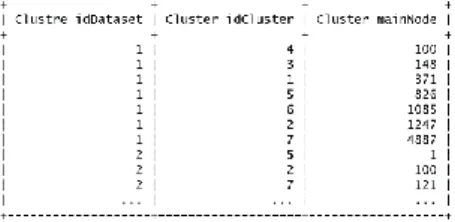
Figure 3 Clusters example output
5) Associate documents and performance measures (Callon’s centrality and density, documents, citations count, and h-index) chosen by the analyst for each cluster. To do this, Queries 9, 10, 12, 13 and 14 must be run. For example, Figure 4 shows a subset of the centrality measures associated with each cluster.
6) Build the evolution map in order to carry out a longitudinal analysis. For this, Query 15 must be run. In this example the Inclusion index formula (see Query 16) has to be set as SIMILARITY-MEASURE. For example, Figure 5 shows the results obtained for the first two consecutive periods.
After applying these steps, all of the data needed to carry out a longitudinal science mapping analysis should be recorded in the database. The data may be used directly and interpreted by the analyst or it may be exported for use by third- party software [9]. To do this, once again standard SQL statements (i.e., Query 17) or PL/SQL procedures may be used. An example of the output generated by this step is seen in Figure 6.
Figure 4
Centrality measure example output
Figure 5
Evolution map example output
Figure 6 Report example output
Concluding Remarks
This paper presents a relational database model for science mapping analysis. This database model was conceived specifically for use in almost all of the stages of a science mapping workflow. The database model was developed as an entity- relations diagram based on the information that is typically present in science mapping studies [9]. The database model also allows for application of the methodology for science mapping analysis proposed in [8]. To validate the proposal, several SQL statements and three PL/SQL procedures were presented.
Finally, it is important to note that one of the most important advantages of this proposal is that it allows for the implementation of a science mapping analysis in an easy, free and cheap way, using only standard SQL statements, which are present in most database management systems.
Acknowledgements
This work was conducted with the support of Project TIN2010-17876, the Andalusian Excellence Projects TIC5299 and TIC05991, and the Genil Start-up Projects Genil-PYR-2012-6 and Genil-PYR-2014-15 (CEI BioTIC Granada Campus for International Excellence).
References
[1] S. Alonso, F. J. Cabrerizo, E. Herrera-Viedma, F. Herrera. “h-index: A Review Focused in Its Variants, Computation and Standardization for Different Scientific Fields”. Journal of Informetrics, 3(4), pp. 273-289, 2009
[2] V. Batagelj, A. Mrvar. “Pajek – Program for Large Network Analysis.
Connections”. 1998
[3] M. Bastian, S. Heymann, M. Jacomy. “Gephi: an Open Source Software for Exploring and Manipulating Networks”. In: Proceedings of the International AAAI Conference on Weblogs and Social Media. 2009 [4] K. Börner, C. Chen, K. Boyack. “Visualizing Knowledge Domains”.
Annual Review of Information Science and Technology, 37, pp. 179-255, 2003
[5] M. Callon, J. P. Courtial, W. A. Turner, S. Bauin. “From Translations to Problematic Networks: An Introduction to Co-Word Analysis”. Social Science Information, 22, pp. 191-235, 1983
[6] M. Callon, J. P. Courtial, F. Laville. “Co-Word Analysis as a Tool for Describing the Network of Interactions between Basic and Technological Research - the Case of Polymer Chemistry”. Scientometrics, 22, pp. 155- 205, 1991
[7] M. J. Cobo, F. Chiclana, A. Collop, J. de Oña, E. Herrera-Viedma. "A Bibliometric Analysis of the Intelligent Transportation Systems Research
based on Science Mapping". IEEE Transactions on Intelligent Transportation Systems, 11(2), pp. 901-908, 2014
[8] M. J. Cobo, A. G. López-Herrera, E. Herrera-Viedma, F. Herrera. “An Approach for Detecting, Quantifying, and Visualizing the Evolution of a Research Field: A Practical Application to the Fuzzy Sets Theory Field”.
Journal of Informetrics, 5(1), pp. 146-166, 2011
[9] M. J. Cobo, A. G. López-Herrera, E. Herrera-Viedma, F. Herrera. “Science Mapping Software Tools: Review, Analysis and Cooperative Study among Tools”. Journal of the American Society for Information Science and Technology, 62, pp. 1382-1402, 2011
[10] M. J. Cobo, A. G. López-Herrera, E. Herrera-Viedma, F. Herrera.
“SciMAT: A New Science Mapping Analysis Software Tool”. Journal of the American Society for Information Science and Technology, 63, pp.
1609-1630, 2012
[11] M. J. Cobo, M. A. Martínez, M. Gutiérrez-Salcedo, H. Fujita, E. Herrera- Viedma. "25 Years at Knowledge-based Systems: A Bibliometric Analysis". Knowledge-Based Systems, 80, pp. 3-13, 2015
[12] N. Coulter, I. Monarch, S. Konda. “Software Engineering as Seen through its Research Literature: A Study in Co-Word Analysis”. Journal of the American Society for Information Science, 49, pp. 1206-1223, 1998 [13] N. J van Eck NJ, L. Waltman. “How to Normalize Co-Occurrence Data?
An Analysis of Some Well-known Similarity Measures”. Journal of the American Society for Information Science and Technology, 60, pp. 1635- 1651, 2009
[14] Elmasri, R.; Navathe, S. B. (2011) Fundamentals of Database Systems (6th ed.) Pearson/Addison Wesley
[15] W. Gänzel. National Characteristics in International Scientific Coauthorship Relations. Scientometrics, 51, pp. 69-115, 2001
[16] J. Hirsch. “An Index to Quantify an Individuals Scientific Research Out- Put”. Proceedings of the National Academy of Sciences, 102, pp. 16569- 16572, 2005
[17] W. W. Hood, C. S. Wilson. “Informetric Studies using Databases:
Opportunities and Challenges”. Scientometrics, 58, pp. 587-608, 2003 [18] M. M. Kessler. “Bibliographic Coupling between Scientific Papers”.
American Documentation, 14, pp. 10-25, 1963
[19] A. G. López-Herrera, E. Herrera-Viedma, M. J. Cobo, M. A. Martínez, G.
Kou, Y. Shi. "A Conceptual Snapshot of the First 10 Years (2002-2011) of the International Journal of Information Technology & Decision Making".
International Journal of Information Technology & Decision Making 11(2), pp. 247-270, 2012
[20] N. Mallig. “A Relational Database for Bibliometric Analysis”. Journal of Informetrics, 4, pp. 564-580, 2010
[21] M. A. Martínez-Sánchez, M. J. Cobo, M. Herrera, E. Herrera-Viedma.
"Analyzing the Scientific Evolution of Social Work Discipline using Science Mapping". Research on Social Work Practice, 5(2), pp. 257-277, 2015
[22] H. F. Moed. “The Use of Online Databases for Bibliometric Analysis”, Proceedings of the First International Conference on Bibliometrics and Theoretical Aspects of Information Retrieval, pp. 133-146, 1988
[23] S. Morris, B. van Der Veer Martens. “Mapping Research Specialties”.
Annual Review of Information Science and Technology, 42, pp. 213-295, 2008
[24] C. Neuhaus, H. Daniel. “Data Sources for Performing Citation Analysis: an Overview”. Journal of Documentation, 64, pp. 193-210, 2008
[25] E. C. M. Noyons, H. F. Moed, A. F. J. van Raan. “Integrating Research Performance Analysis and Science Mapping”. Scientometrics, 46, 591-604, 1999
[26] Orestes Appel, Francisco Chiclana, Jenny Carter. "Main Concepts, State of the Art and Future Research Questions in Sentiment Analysis". Acta Polytechnica Hungarica 12 (3), pp. 87-108, 2015
[27] H. P. F. Peters, A. F. J. van Raan. “Structuring Scientific Activities by Coauthor Analysis an Exercise on a University Faculty Level”.
Scientometrics, 20, pp. 235-255, 1991
[28] Popescu-Bodorin, N. and Balas, V. E. "Fuzzy Membership, Possibility, Probability and Negation in Biometrics". Acta Polytechnica Hungarica 11 (4), pp. 79-100, 2014
[29] P. Shannon, A. Markiel, O. Ozier, N. Baliga, J. Wang, D. Ramage, N.
Amin, B. Schwikowski, T. Ideker. “Cytoscape: A Software Environment for Integrated Models of Biomolecular Interaction Networks”. Genome Research, 13, 2498-2504, 2003
[30] H. Small. “Co-Citation in the Scientific Literature: a New Measure of the Relationship between Two Documents”. Journal of the American Society for Information Science, 24, pp. 265-269, 1973
[31] H. Small. “Visualizing Science by Citation Mapping”. Journal of the American Society for Information Science, 50, pp. 799-813, 1999
[32] H. Yu, M. Davis, C. Wilson, F. Cole. “Object-Relational Data Modelling for Informetric Databases”. Journal of Informetrics, 2, pp. 240-251, 2008 [33] L. Zadeh. “Fuzzy Sets”. Information and Control, 8, pp. 338-353, 1965 [34] L. Zadeh. “Is There a Need for Fuzzy Logic?” Information Sciences, 178,
pp. 2751-2779, 2008