P The Impact of the Institutional Factors in the Public Sphere on Export in OECD Countries

(1)

P

Alper Ozmen – Tufan Saritas

The Impact of the Institutional Factors in the Public Sphere

on Export in OECD Countries

S^ummary: As it is known, export is a positive economic phenomenon that is desired to be realized for all countries. From this point of view the effect of institutional factors in the public sphere on export was investigated in 36 OECD countries for the period between 2002-2018. Four different models were established in the study and export was defined as the dependent variable in all models. In the first model it is determined that there is a negative relationship between the control of corruption and export. In the second model it was determined that there is an inverse relationship between regulatory quality and export.

In the third model it is observed that there is a similar relationship between political stability and exports. In the fourth model that investigates the possible effect of the rule of law on exports there was no statistically significant relationship between the relevant variables.

KeywordS: public administration, institutional factors, export, panel data analysis.

JeL-codeS: H83, F10, G18, G19

doI: https://doi.org/10.35551/PFQ_2021_1_7

Public administration policies and political decisions cannot be considered seperately from economic developments. Capital investments, planning of manpower, distribution of resources, economic cooperation, role of the private sector are planned by governments, with taking into consideration the global and national economic order. in this study, an answer is searched for the question to which extent parameters such as the control of corruption, regulatory quality, political stability and the rule of law, among the institutional factors in the public sphere affects the export.

As it is known, corruption is defined as the abuse of public service for private interests. it has the ability to stabilize or destabilize the political system because of its structure (Farzanegan and Witthuhn, 2017:

48). There is a worldwide increasing concern about corruption, which is now universal it is closely related to the idea that it will hinder the economic development process and to play a central role in politics. today, not only the public and private sectors, but also non- profit organizations and charities in developed and developing countries are subject to corruption. (Myint, 2000: 33). Beyond any doubt, corruption provokes inefficiency instrumentally. Waste of resources, decrease E-mail address: aozmen@ogu.edu.tr

tufansaritas@kmu.edu.tr

(2)

in per capita income, negative shift in employment are the main ones of that fact.

Corruption also affects negatively the tax revenues and service quality by weakening trust in public officials (Rose, 2018: 220).

Regulatory quality is a complex concept that has several parameters on its own. its normative dimension stands out more. it includes setting goals for management, clarifying the scope of public interventions, impartiality, good governance and transparent regulation (Radaelli and Francesco, 2004).

it is within the scope of regulatory quality that governments encourage private sector development, formulate the policies that facilitate private sector initiatives (Nistotskaya and Cingolani, 2015: 10; info.worldbank.org, 2020).

For economic growth, social welfare and environmental protection it is needed to establish rules. However, rules can sometimes be costly, both economically and socially. What is needed to be done is to create a more efficient and cost-effective regulatory quality system without removing existing rules. in that way, governments improve existing rules by drafting good and new rules. By removing individual rules that contradicts with each other, well prepared regulations are meant to be subject of the system parts (OeCd, 2008: 1).

Political stability is a necessary condition for the optimal functioning of the economy.

economic growth, income inequality, inflation, the level of poverty, fiscal and monetary policy decisions are variables that affect political stability. in the short and long term, political stability supports economic growth, provided by private representatives and government policy decisions (Cervantes and Villasenor, 2015: 79-81). Political instability has a negative impact on economic growth. The reason of this is that it disrupts market activities and working relations by negatively affecting production. Besides, in

times of political instability, the investment level will be low (Radu, 2015: 752).

Rule of law expresses the authority of legal rules over government actions and the behavior of individuals. Hence, it is the antithesis of tyrannical rule that both government and individuals are bound by the law (Valcke, 2020). The law is equitable; it is stable and predictable; it applies equally to everyone in similar circumstances; superior to all members of society, including government officials with legislative, executive and judicial powers (Stein, 2009: 302).On that sense, it is a system that tries to protect the rights of citizens from the arbitrary acts and abuses of government power (Yu and Guernsey, 2020).

LItErAturE

One of the first studies to examine the possible relationship between corruption and foreign trade was carried out by Krueger (1974). in his study, Krueger emphasized the importance of having an import license for companies dealing with foreign trade in an environment where imports are restricted by quantity restrictions and argued that companies may compete with each other and even do unlawful things in order to obtain this license.

Bhagwati (1982) argues in his study that, in a competitive economic environment, businesses can try to circumvent tariffs and resort to illegal means such as customs smuggling. According to him, these enterprises do not contribute significantly to production, but by developing close relations with the government, they set out to obtain rent and increase their income.

Nitsch and Schumacher (2004) investigated the impact of terrorism on international trade in their study. According to the findings of the study, which bounded with the 1960-1993 period and covers more than 200 countries,

(3)

it was observed that terrorist acts narrow the volume of foreign trade.

Clarke (2005) conducted a research on the factors determining the export performance of enterprises operating in the manufacturing industry in his study, which included 8 African countries. in his study, where he collected data through surveys covering the years 2002 and 2003, he found that manufacturing firms were less likely to export in countries with restrictive trade and customs regulations and poor customs administration.

Iwanow and Kirkpatrick (2007) studied 78 countries for the period of 2000-2004 and investigated the relationship between facilities provided for trade, regulatory quality and export performance. in their findings, they determined that a 10 percent improvement in trade facilitation would provide a 5 percent increase in exports. in additionto this; While trade facilitation can contribute to improving export performance, it confirms that improvements in regulatory quality as well as the quality of basic transport and communication infrastructure are more important to export performance and accelerate export growth.

Dutt and Traca (2010) examined the relationship between corruption and foreign trade in their study within the context of extortion effect and evasion effect. According to the authors; Corrupting customs officials in the importing country taking bribes from exporters (extortion effect); and subsequently, if it allows exporters to avoid tariff barriers, corruption can increase trade. (evasion effect).

in the empirical findings of the study, especially in the case of high tariffs, it has been observed that the extortions taken by customs officials and causing corruption increased foreign trade.

Musila and Sigué (2010) investigated the impact of corruption on foreign trade in African countries for the period between 1998-2007. in the empirical findings of this

study, they observed that corruption affects foreign trade negatively.

Yu et al. (2015) investigated the relationship between trade, trust and the rule of law in 16 european countries for the period between 1996-2009. in the findings obtained; it is emphasized that the positive effect of trust on trade is determined by the quality of the rule of law. Additionally, it has been observed that when the rule of law in the importing country increases compared to the exporting country, the effect of trust on trade decreases.

in the study conducted by Gezikol and Tunahan (2018), in the low-income country group for the period between 1995-2015, it has been observed that the increase in exports resulted in increased corruption. in the low-middle income country group, it was determined that the increase in imports and exports again resulted in increased corruption.

in Soyyiğit and Doğan (2020) studies, for the period between 2000-2017, in the countries of the Commonwealth of independent States;

They investigated the relationship between institutional factors, exports and foreign direct investments. in the empirical findings obtained; A one-sided causality relationship from the rule of law to export and political stability has been identified. in addition, a unidirectional causality relationship has been observed from the government’s effectiveness to exports and foreign direct investments.

in the next part of the study, at first place, brief information will be given about the data and method used in the analysis. Afterwards;

The research findings will be reported and the conclusion part will take place lastly.

DAtA AnD MEtHOD

in this study, the effects of corruption control, political stability, regulatory quality and the rule of law on exports, which are among the

(4)

institutional factors that have an impact on the public sphere for the period 2002-2018 in the context of 36 OeCd countries, were investigated using panel data analysis. The data used in the study are shown in the Table 1 below with their sources.

As can be seen in the table above, all of the series were obtained from the World Bank.

Logarithmic transformation was applied to dLeXP and dLGdP series that did not have negative values, and other series that had negative values in observations of some years were added to the model in their original form.

to explain the variables representing institutional factors; the corruption control index, in the context of all forms of corruption, regardless of whether they are minor or largely, it measures perceptions of the extent to which public power is used for private gain, as well as the administration of the state by the elite and private interests. Regulatory quality index;

it measures perceptions of the government’s ability to form and implement solid policies that allow and encourage private sector development. The political stability index measures perceptions of political stability and the absence of violence, political instability, including terrorism, and / or the possibility

of politically motivated violence. The rule of law index, on the other hand, measures the perceptions of the representatives regarding how much they trust and obey the rules of the society and especially the contract practices, property rights, the quality of the police and courts, and the possibility of crime and violence. For these four indices of institutional factors, the estimate gives the country’s score between approximately –2.5 and 2.5. in addition, descriptive statistics for all series are reported in the Table 2.

Since the data set used in this study is a panel data set, panel data analysis was preferred as a method. First, unit root test was applied to determine the stationarities of the series. Second generation panel unit root tests can make consistent estimates in series when cross-sectional dependency is in question. For this reason, firstly, the presence of cross-sectional dependency in series was investigated. Because in the panel data set used in the study N>T, cross section dependency was investigated with the Peseran Cd LM test proposed by Peseran (2004). if the probility value obtained as a result of the Peseran Cd LM test is less than 5% significance level, the H0 hypothesis, which states that there is no

Table 1 Data anD SourceS

Variable code Variable name Source

DLEXP Exports of goods and services (constant 2010) WDI

DCOr Control of Corruption Index WDI

DrEG regulatory Quality Index WDI

DPOL Political Stability and Absence of Violence/terrorism Index WDI

DLAW rule of Law Index WDI

DLGDP GDP (constant 2010 uS$) WDI

DFDI Foreign direct investment, net inflows (% of GDP) WDI

Source: own edited

(5)

cross-sectional dependency, is rejected, and the H1 hypothesis expressing the presence of cross-section dependence is accepted. if the probility value is greater than 5% significance level, the H0 hypothesis is accepted and the H1 hypothesis is rejected.

in the case of cross-sectional dependency in the series, the Peseran CiPS unit Root test, which is one of the second generation unit root tests and can make consistent predictions under the assumption of cross-section dependency, has been investigated for the stationarities of the series. After determining the stationarities, the differences of the non- stationary series were taken and the models were established.

in the F test test of the models, if the probility value of the F test is less than 5% significance level, the hypothesis ‘H0:

Classical model is suitable’ is rejected and the alternative ‘H1: Classical model is not suitable’ hypothesis is accepted. Therefore, it is understood that unit/time effective models are available in this case. if the probility value of the F test is greater than 5% significance level, the hypothesis ‘H0: Classical model is suitable’ is accepted and the alternative ‘H1:

Classical model is not suitable’ hypothesis is rejected. in other words, in this case, it is

decided that unit/time effective models are not available, instead the classical model is suitable.

Hausman (1978) test was used to determine the fixed and random effects in the models. if the probility value of the Hausman test is statistically less than 5%

significance level, the hypothesis ‘H0: The difference between the parameters is not systematic’ is rejected and the alternative

‘H1: The difference between the parameters is systematic’ hypothesis is accepted. in other words, it is understood that fixed effects model is valid in models. if the probility value of Hausman test is statistically greater than 5% significance level, the hypothesis

‘H0: The difference between the parameters is not systematic’ is accepted and the alternative

‘H1: The difference between the parameters is systematic’ hypothesis is rejected. in other words, it is understood that the random effects model is valid in models.

This method has the ability to make consistent estimates even in the presence of heteroskedasticity and autocorrelation problems in the model (Yerdelen tatoğlu, 2018: 101). in addition, there are versions of this method that can be used in both random effect models and fixed effect models. in the Table 2 Summary StatiSticS about Data

Variable mean min. max. Std. Dev. obs

DLEXP 0.0448 –0.2669 0.3312 0.0643 576

DCOr –0.0066 –0.3705 0.3380 0.0945 576

DrEG –0.0001 –0.3041 0.5722 0.0936 576

DPOL –0.0215 –0.7468 0.5526 0.1467 576

DLAW –0.0015 –0.2577 0.2542 0.0710 576

DLGDP 26.6891 23.1230 30.5134 1.5907 576

FDI 5.0513 –58.3229 86.5891 10.7765 612

(6)

study, Generalized Least Squares Method was used considering these versions.

different tests were used for fixed and random effect models in determining heteroskedasticity problem in models.

Modified Wald test, which is recommended to be used in fixed effect models, was preferred in determining the heteroscedasticity problem for fixed effect models. if the probility value of this test is statistically less than 5% significance level; The hypothesis of ‘H0: Variance is constant with respect to units’ is rejected and the alternative ‘H1: Variance is not constant with respect to units’ hypothesis is accepted.

in other words, it is concluded that there is a heteroscedasticity problem in the model.

if the Probility value is statistically higher than 5% significance level; The hypothesis

‘H0: Variance is constant with respect to units’

is accepted and the alternative ‘H1: Variance is not constant with respect to units’ hypothesis is rejected. in other words, it is decided that there is no heteroscedasticity problem in the model.

For determination of the heteroscedasticity problem, if random effect models are valid The tests developed by Levene (1960) and Brown and Forsythe (1974) were used. if the probility value of the relevant tests for different critical values (1%, 5%, 10%) is statistically lower than the 5% significance level, the H0 hypothesis, which states that there is no heteroskedasticity problem, is rejected, and the H1 hypothesis expressing that there is a problem of heteroskedasticity is accepted. if the Probility value is statistically higher than 5% significance level; The H0 hypothesis, which states that there is no heteroskedasticity problem, is accepted, and the H1 hypothesis, which states that there is a heteroskedasticity problem, is rejected.

Bharagava, Franzi, and Narendranathan’s (1982) Durbin-Watson test and Baltagi and Wu’s (1999) best invariant test (LBi)

were used to determine the autocorrelation problem in models. if the statistical value of both tests is less than 2, it is concluded that the autocorrelation problem in the model is important. if the statistic value is greater than 2; it is decided that the autocorrelation problem in the model is not important.

As mentioned before, the Generalized Least Squares Method has the ability to make consistent estimates even under the presence of autocorrelation and heteroskedasticity.

However, in the study, consistent estimators were used to eliminate the related problems in the models. in the models where the fixed effect model is valid, the consistent estimator developed by Driscoll and Kraay (1998), which is suitable for fixed effect models, is preferred.

The reason for choosing this estimator is that it can be used both in fixed effect models and if the N> t condition is valid in the panel data set. Random effect models are; The consistent estimator, which was developed by Arellano (1987), Froot (1989) and Rogers (1993), was used in the random effects model.

Four different models were used in the study. Representing export in all models, dLeXP series is the dependent variable.

dLGdP series representing growth and Fdi series representing foreign direct investment inflows are control variables. installed models are as follows:

DLEXP_it=β₀+β₁ DCOR+β₂ DLGDP+β₃ FDI+ε_it (1) DLEXP_it=β₀+β₁ DREG+β₂ DLGDP+β₃ FDI+ε_it (2) DLEXP_it=β₀+β₁ DPOL+β₂ DLGDP+β₃ FDI+ε_it (3) DLEXP_it=β₀+β₁ DLAW+β₂ DLGDP+β₃ FDI+ε_it (4)

in the first model, the dCOR series representing the control of corruption;

in the second model, the dReG series representing regulatory quality;

in the third model, the effect of the dPOL

(7)

series representing political stability and the dLAW series representing the rule of law;

in the fourth model on the dLeXP series representing exports, were investigated.

Analysis results will be reported in the next part of the study. Then it will continue with the results section.

AnALySIS rESuLtS

in the study, before starting panel data analysis, relevant tests were used to test the unit roots of the series. As is known, it is suggested to use second generation unit root tests in case of structural break in series. Since N> t in the data set used in the study, the Peseran Cd LM test recommended by Peseran (2004) was used to determine the cross-sectional dependency of the series. information on test results is shown in the Table 3 below.

As can be seen in the table above, it is understood that the probility values of all models are statistically less than 5%

significance level. in other words, the H0 hypothesis, which states that there is no cross- sectional dependency, was rejected, and the H1 hypothesis, which expresses the presence of cross-section dependence, was accepted.

Since it was understood that there is cross section dependency in models, it was decided to use one of the second generation unit root tests considering the cross section dependency.

in this context, the Peseran CiPS test, one of the second generation unit root tests, was preferred and the stationarity results for the series are reported in the Table 4 below.

As seen in the above table of the Peseran CiPS unit root test results, only Fdi series are stationary in i (0); all other series are stationary in i (1). After the non-stationary series in i (0) were made stable in i (1) by taking their first differences, the models were established and the estimation phase was started. The estimation results made with the generalized least squares method are reported in the Table 5 below.

As seen in the table below, the dLeXP series representing exports in all models is the dependent variable. in the results belonging to Model-1;

• dCOR series representing the control of corruption, with a coefficient of -0.0375, statistically negative at 10% significance;

• dLGdP series representing growth, with 1.3881 coefficient, the Fdi series representing foreign direct investments positively at 1% significance level, and

• dLeXP series representing exports with a statistically significant level of 5%, with a coefficient of 0.0004.

in other words, it is seen that there is an inverse relationship between the control of corruption and exports. in other words, as the control of corruption increases, exports decrease and as the control of corruption decreases, exports increase.

Table 3 PeSeran cD Lm teSt reSuLtS

model-1 model-2 model-3 model-4

Coef.

(Prob.)

16.384 (0.0000)

18.726 (0.0000)

18.456 (0.0000)

20.439 (0.0000) Source: own edited

(8)

Table 4 PeSeran ciPS unit root teSt reSuLtS

Variable model test Stat. critival Values

%10 %5 %1

DLEXP Constant –1.625 –22.11 –22.20 –22.36

Constant Linear tr. –2.142 –2.63 –2.71 –2.85

DLEXP Constant –3.275 –2.11 –2.20 –2.36

DCOr Constant –2.144 –2.11 –2.20 –2.36

DCOr Constant –3.862 –2.11 –2.20 –2.36

DrEG Constant –1.572 –2.11 –2.20 –2.36

DrEG Constant –4.250 –2.11 –2.20 –2.36

DPOL Constant –2.034 –2.11 –2.20 –2.36

DPOL Constant –4.332 –2.11 –2.20 –2.36

DLAW Constant –1.833 –2.11 –2.20 –2.36

DLAW Constant –4.054 –2.11 –2.20 –2.36

DLGDP Constant –1.243 –2.11 –2.20 –2.36

DLGDP Constant –2.919 –2.11 –2.20 –2.36

FDI Constant –3.447 –2.11 –2.20 –2.36

(9)

in the results for Model-2;

• dReG series representing regulatory quality, with a coefficient of -0.0535, statistically negative at 5% significance level;

• dLGdP series representing growth, with a coefficient of 1.3610, statistically positive at 1% significance level

• and the Fdi series representing foreign

direct investments affects the dLeXP series, which represents exports positively at a 10% significance level with a coefficient of 0.0004.

in other words, it is seen that there is an inverse relationship between regulatory quality and export. in other words; As the regulatory quality increases, exports decrease and as the regulatory quality decreases, exports increase.

Table 5 eStimation reSuLtS (GeneraLizeD LeaSt SquareS)

Depended Variable: DLeXP

DCOr –0.0375*

(0.0740)

– – –

DrEG – –0.0535*

(0.0100)

– –

DPOL – – 0.0387*

(0.0030)

–

DLAW – – – –0.0061*

(0.8270)

DLGDP 1.3881*

(0.0000)

1.3610*

(0.0000)

1.3274*

(0.0000)

1.3437*

(0.0000)

FDI 0.0004*

(0.0390)

0.0004*

(0.0530)

0.0004*

(0.0480)

0.0004*

(0.0570)

Fixed 0.0102*

(0.0000)

0.0115*

(0.0000)

0.0103*

(0.0000)

0.0119*

(0.0000)

number of Obs 576 576 576 576

number of Country 36 36 36 36

r² 47 48 48 47

F test Stat. (Prob.) 2.15 (0.0002)

2.08 (0.0004)

2.11 (0.0003)

2.10 (0.0003) Hausman test

Stat. (Prob.)

14.82 (0.0020)

7.02 (0.0713)

5.83 (0.1204)

5.68 (0.1284)

Model Fixed Effect random Effect random Effect random Effect

*Note: Values in parantheses are probility values, others are coefficients.

(10)

in the results belonging to Model-3;

• dPOL series representing political stability, with a coefficient of 0.0387, statistically positive at 1% significance level;

• dLdGP series representing growth, with a coefficient of 1.3274, statistically positive at 1% significance level

• and Fdi series representing foreign direct investments, with a coefficient of 0.0004, positively affects the dLeXP series representing exports at a statistically significant level of 5%.

in other words, there is a directly related relationship between political stability and exports. As the political stability increases, exports increase and as the political stability decreases, exports decrease.

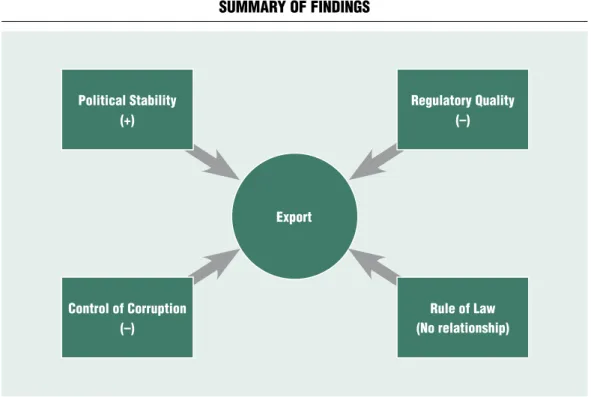
in the results belonging to Model-4; it is seen that the dLAW series representing the rule of law does not have a statistically significant effect on exports. However, with the coefficient of 1.3437, the dLGdP series representing growth, statistically, at the level of 1% significance and Fdi series representing foreign direct investments with a coefficient of 0.0004, with a statistical significance of 10%, positively affects the dLeXP series representing export. The findings are shown in Figure 1.

The table below shows the results of the diagnostic tests for the models. different tests were used to determine autocorrelation and heteroskedasticity problems, depending on whether the models are fixed and randomly effective models. As can be seen in the Table 6 below, it is understood that there are autocorrelation and heteroskedasticity problems in all models. Consistent estimators were consulted to solve the related problems and the results were reported in the relevant table showing the results of the consistent estimators.

Consistent estimators were used to eliminate heteroskedasticity and autocorrelation

problems in the models and the results are reported in the Table 7 below. Since the fixed effects model is valid in Model-1 and the panel data set used is shaped as N> t, the consistent estimator developed by driscoll and Kraay (1998) was used for this model. As can be seen in the results obtained for Model-1;

• dCOR series representing the control of corruption, with –0.0375 coefficient, statistically negative at 1% significance level;

• representing growth, the dLGdP series, with a coefficient of 1.3881, positively

• and Fdi series representing foreign direct investments, with a coefficient of 0.0004, positively affects the dLeXP series representing exports at a statistically significant level of 1%.

in other words, there is an inverse relationship between corruption control and export. As the control of corruption increases, exports decrease and conversely, as the control of corruption decreases, exports increase.

in order to overcome the heteroskedasticity and autocorrelation problems in Model-2, the current version of the consistent estimator in the random effects model, developed by Arellano (1987), Froot (1989) and Rogers (1993), was used. As can be seen in the Table 7, in the findings obtained;

• dReG series representing regulatory quality, with a coefficient of –0.0535, statistically negative at 1%;

• with the coefficient of 1.3610 of the dLGdP series representing growth, statistically positive at 1% significance level

• and the Fdi series representing foreign direct investments, with a coefficient of 0.0004, positively affects the dLeXP series representing exports at a statistically significant level of 1%.

in other words, there is an inverse relationship between regulatory quality and

(11)

Table 6 DiaGnoStic teStS reSuLtS for moDeLS

Model Fixed Effect random Effect random Effect random Effect

Modified Wald test Stat.

(Prob.)

774.63 (0.0000)

– – –

Baltagi-Wu test Stat. 1.9825 1.9873 1.9852 1.8959

Durbin- Watson test Stat. 1.9012 1.9018 1.9066 1.9777

Critival Values (Levene, Brown ve Forsthe test Stat. & Prob.)

– 0.01 = 2.0563 (0.0004) 0.05 = 1.7894

(0.0041) 0.10 = 1.9401 (0.0012)

0.01 = 2.0563 (0.0004) 0.05 = 1.7894

(0.0041) 0.10 = 1.9401 (0.0012)

0.01 = 2.0563 (0.0004) 0.05 = 1.7894

(0.0041) 0.10 = 1.9401 (0.0012) Source: own edited

Figure 1 Summary of finDinGS

export Political Stability

(+)

regulatory quality (–)

rule of Law (no relationship) control of corruption

(–)

(12)

export. in other words, as the regulatory quality increases, exports decrease and conversely, as the regulatory quality decreases, exports increase.

in order to overcome the heteroskedasticity and autocorrelation problems in Model-3, the consistent estimator, which was developed by Arellano (1987), Froot (1989) and Rogers (1993), was used in the random effects model.

As seen in the table above;

• with the coefficient 0.0387 of the dPOL series representing political stability, the statistically positive direction at 1%

significance level;

• with the coefficient of 1.3274 of the dLGdP series representing growth, statistically positive at 1% significance leveland and

• the Fdi series representing foreign direct investments, with a coefficient of 0.0004, positively affects the dLeXP series representing exports at a statistically significant 1% level.

in other words, there is a similar relationship between political stability and exports. As the political stability increases, exports increase and as the political stability decreases, exports decrease.

Table 7 eStimation reSuLtS (conSiStent eStimatorS)

Depended Variable: DLeXP

DCOr –0.0375*

(0.0010)

– – –

DrEG – –0.0535*

(0.0080)

– –

DPOL – – 0.0387*

(0.0060)

–

DLAW – – – –0.0061*

(0.8280)

DLGDP 1.3881*

(0.0000)

1.3610*

(0.0000)

1.3274*

(0.0000)

1.3437*

(0.0000)

FDI 0.0004*

(0.0080)

0.0004*

(0.0030)

0.0004*

(0.0050)

0.0004*

(0.0050)

Fixed 0.0103*

(0.1000)

0.0115*

(0.0010)

0.0130*

(0.0010)

0.0119*

(0.0010) Method Driscoll-Kray Consistent Estimators Consistent Estimators Consistent Estimators

r² 47 48 48 47

number of Obs 576 576 576 576

number of Country 36 36 36 36

Note: *Values in parantheses are probility values, others are coefficients.

(13)

in order to overcome the heteroskedasticity and autocorrelation problems in Model-4, the consistent estimator, which was developed by Arellano (1987), Froot (1989) and Rogers (1993), was used in the random effects model.

As seen in the table above;

• the dLGdP series, which represents growth from the control variables, with a coefficient of 1.3437, statistically positive at 1% significance level and

• the Fdi series representing foreign direct investments, with a coefficient of 0.0004, positively affects the dLeXP series representing exports at a statistically significant level of 1%.

On the other hand, the dLAW series representing the rule of law could not have a statistically significant effect on exports.

COnCLuSIOn

in this study, for the period of 2002-2018 in the context of 36 OeCd countries, the effects of corruption control, political stability, regulatory quality and the rule of law, which are among the institutional factors that affect the public sphere, on exports were investigated using panel data analysis. Four different models were established in the study, and export was defined as the dependent variable in all models.

in Model-1, the effect of control of corruption on exports has been investigated.

Growth and foreign direct investment inflow are included in the model as control variables.

in the estimation made by the generalized least squares method, in the results belonging to Model-1;

• dCOR series representing the control of corruption, with a coefficient of -0.0375, statistically negative at 10% significance level;

• dLGdP series representing growth,

with a coefficient of 1.3881, statistically positive at 1% significance level, and

That is to say, it is seen that there is an inverse relationship between the control of corruption and exports. in other words, as the control of corruption increases, exports decrease and as the control of corruption decreases, exports increase.

Heteroskedasticity and autocorrelation problems were detected in Model-1. Since fixed effects are valid in the model and the panel data set used is formed as N> t, the consistent estimator developed by driscoll and Kraay (1998) was used to solve the related problems. in the results obtained;

• dCOR series representing the control of corruption, with –0.0375 coefficient, statistically negative at 1% significance level;

• representing growth, the dLGdP series, with a coefficient of 1.3881, positivelyand Fdi series representing foreign direct investments, with a coefficient of 0.0004, positively affects the dLeXP series representing exports at a statistically significant 1% level.

Although the result did not change, it was observed that there was an increase in statistical significance.

in Model-2, the effect of regulatory quality on exports has been investigated. Again, growth and foreign direct investment inflows are included in the model as control variables.

in the estimation made with the generalized least squares method, in the results of Model-2;

• dReG series representing regulatory quality, with a coefficient of -0.0535, statistically negative at 5% significance level;

(14)

• dLGdP series representing growth, with a coefficient of 1.3610, statistically positive at 1% significance level and

• Fdi series, which represents foreign direct investments, affects the dLeXP series, which represents exports positively at a 10% significance level with a coefficient of 0.0004.

Particularly, it is seen that there is a reverse relationship between regulatory quality and export. That is; As the regulatory quality increases, exports decrease and as the regulatory quality decreases, exports increase.

Heteroskedasticity and autocorrelation problems were detected in Model-2. Since the random effects are valid in the model, the version of the consistent estimator, which is valid in the random effects model, was used to solve the related problems. in the findings obtained;

• dReG series representing regulatory quality, with a coefficient of –0.0535, statistically negative at 1%;

• with the coefficient of 1.3610 of the dLGdP series representing growth, statistically positive at 1% significance level and

• the Fdi series representing foreign direct investments, with a coefficient of 0.0004, positively affects the dLeXP series representing exports at a statistically significant 1% level. Although the result has not changed, it is seen that there is an increase in statistical significance.

in Model-3, the effect of political stability on exports has been investigated. Growth and foreign direct investment inflow are included in the model as control variables. in the findings obtained;

• dPOL series representing political stability, with a coefficient of 0.0387, statistically positive at 1% significance level,

• dLdGP series representing growth,

with a coefficient of 1.3274, statistically positive at 1% significance level and

• Fdi series representing foreign direct investments, with a coefficient of 0.0004, positively affects the dLeXP series representing exports at a statistically significant level of 5%.

in other words, there is a similar relationship between political stability and exports. As the political stability increases, exports increase and as the political stability decreases, exports decrease.

Heteroskedasticity and autocorrelation problems were detected in Model-3. Since random effects are valid in the model, the version of the consistent estimator, which is valid in the random effects model, has been used to solve the related problems. in the results obtained;

• with the coefficient 0.0387 of the dPOL series representing political stability, statistically positive direction at 1%

significance level;

• with the coefficient of 1.3274 of the dLGdP series representing growth, statistically positive at 1% significance leveland

• the Fdi series representing foreign direct investments, with a coefficient of 0.0004, positively affects the dLeXP series representing exports at a statistically significant 1% level.

Although the result did not change, it was observed that there was an increase in statistical significance.

in Model-4, the effect of the rule of law on exports has been investigated. Growth and foreign direct investment inflow are included in the model as control variables. in the findings; it is seen that the dLAW series representing the rule of law does not have a statistically significant effect on exports.

However, with the coefficient of 1.3437, the dLGdP series representing growth,

(15)

statistically, at the level of 1% significance and Fdi series, which represents foreign direct investments, positively affects the dLeXP series representing exports with a statistically significant level of 10% with a coefficient of 0.0004.

Heteroskedasticity and autocorrelation problems were detected in Model-4. Since the random effects are valid in the model, the version of the consistent estimator, which is valid in the random effects model, was used to solve the related problems. in the results obtained;

• the dLGdP series, which represents growth from the control variables, with a coefficient of 1.3437, statistically positive at 1% significance level and

However, the dLAW series representing the rule of law could not have a statistically significant effect on exports.

The economic policies implemented by the governments can create some restrictions on foreign trade in terms of both their own interests and the sanctions of international law and international organizations. On the other hand, firms often tend to put their own interests ahead of those of national and international institutions and organizations.

due to the restrictions of governments and international organizations, companies sometimes have difficulty in exporting.

Therefore, as can be seen in the findings of this study, export and control of corruption have a negative relationship. Bhagwati (1982) points out to this finding in his study and argues that in an economic environment

where competition is fierce, businesses may try to circumvent customs tariffs and resort to some illegal means such as customs smuggling.

in addition, in the study of Bhagwati (1982), it is argued that these enterprises, although not contributing significantly to production, started to obtain rent and increase their income by developing close relations with the government. to put it more clearly, these enterprises also demand the stable continuation of the government with which they have an association. Because the stable continuation of the current foreign trade of these enterprises depends on the ability of this government in the country to remain in power with political stability. in our study, a similar relationship was found between political stability and exports, confirming this relationship.

iwanow and Kirkpatrick (2007) empirically observed that factors that facilitate trade in regulatory quality have a positive effect on export performance. in our study, we found that there is an invers relationship between regulatory quality and export. in other words, as the regulatory quality increases, public sanctions and legal regulations on exports increase. Therefore, an opposite relationship may arise between regulatory quality and exports as exports become difficult. This finding in our study is similar to that found in the studies of iwanow and Kirkpatrick.

Németh et al. (2019), in some studies such as, attention is drawn to the issue of the reliability of indices measuring corruption. in these studies, it is emphasized that corruption indexes may not reflect the truth. For this reason, it should be noted that we are more skeptical about the corruption findings in our study compared to other findings.

(16)

References Arellano, M. (1987). Computing Robust Standart errors for Within-Groups estimators.

Oxford Bulletin of Economics and Statistics, 49(4), pp.

431-434

Bhagwati, J. N. (1982). directly unproductive, Profit-Seeking (duP) Activities. Journal of Political Economy, 90(5), pp. 988-1002

Baltagi, B. H. & Wu, P. X. (1999). unequally Spaced Panel data Regressions with AR(1) disturbances’. Econometric Theory, 15, pp. 814-823

Bhargava, A., Franzini, L. & Narendranathan, W. (1982). Serial Correlation and Fixed effect Models. The Review of Economic Studies, 49, 533-549

Brown, M. B. & Forsythe, A. B. (1974). The Small Sample Behavior of Some Statistics Which test the equality of Several Means. Technometrics, 16, 129-132

Cervantes, Rosario & Jorge Villasenor (2015). Political Stability and economic Growth:

Some Considerations, Journal of Public Governance and Policy: Latin American Review, 1(1), pp. 77-100

Clarke, George R. G. (2005). Beyond tariff and Quotas: Why don’t African Manufacturing enterprises export More? World Bank Policy Research, Working Paper No: WPS3617

driscoll J. C. & Kray, A. C. (1998). Consistent Covariance Matrix estimation with Spatially dependent Panel data. Review of Economics and Statistics, 80, pp. 549-560

dutt, P. & traca, d. (2010). Corruption and Bilateral trade Flows: extortion or evasion?. The Review of Economics and Statistics, 92(4), pp. 843- 860

Farzanegan, M. R. & S. Witthuhn (2017).

Corruption and political stability: does the youth bulge matter? European Journal of Political Economy, 49, pp. 47-70

Froot, K. A. (1989). Consistent Covariance Matrix estimation with Cross-Sectional dependence and Heteroskedasticity in Financial data. Journal of Financial and Quantitative Analysis, 24, pp.

333-355

Gezikol, B. & tunahan, H. (2018). Algılanan Yoksulluk ile dış ticaret ve doğrudan Yabancı Yatırım Arasındaki İlişkinin uluslararası endeksler Bağlamında ekonometrik Analizi, Alphanumeric Journal, 6(1), pp. 117-132

iwanow, t. & Kirkpatrick, C. (2007). trade Facilitation, Regulatory Quality and export Performance. Journal of International Development, 19, pp. 735-753, info.worldbank.org>wgl>pdf, e.t.:

10. 09. 2020

Krueger, A. O. (1974). The Political economy of the Rent-Seeking Society. The Economic Review, 64(3), pp. 291-303

Levene, H. (1960). Robust tests for equality of Variances. Olkin i., Ghurye G., Hoeffding W., Madow W. G. ve Mann H. B. (ed.), Contributions to Probability and Statistics (pp. 278-292), Stanford California: Stanford university Press

Musila, J. W. & Sigué, S. P. (2010). Corruption and international trade: An empirical investigation of African Countries. World Economy, 33(1), pp.

129-146

Myint, u. (2000). Corruption: Causes, Consequences and Cures, Asia-Pacific Development Journal, 7(2), pp. 33-58

(17)

Németh, e., Vargha, B. t. & Palyi, K. t.

(2019). The Scientific Reliability of international Corruption Rankigs. Public Finance Quarterly, 64(3), pp. 319-336,

https://doi.org/10.35551/PFQ_2019_3_1

Nistotskaya, Marina & Luciana Cingolani (2015). Bureaucratic Structure, Regulatory Quality, and entrepreneurship in a Comparative Perspective:

Cross-Sectional and Panel data evidence, Journal of Public Administration Research and Theory, 16, pp. 1-25

Nitsch, V. & Schumacher, d. (2004). terrorism and international trade: An emprical investigation.

European Journal of Political Economy, 20, pp.

423-433

Peseran, M. H. (2004). General diagnostic tests for Cross Section dependence in Panels. Working Paper, university of Cambridge, united Kingdom

Radaelli, Cladio M. & Fabrizio de Francesco (2004). indicators of Regulatory Quality: Final Report, Centre for european Studies, university of Bradford, Luxembourg

Radu, Madalina (2015), Political Stability - a Condition for Sustainable Growth in Romania?, Procedia Economics and Finance, 30, pp. 751-757

Rogers, W. H. (1993). Regression Standart errors in Clustered Samples. Stata Technical Bulletin, 3, pp. 88-94

Rose, Jonathan (2018). The Meaning of Corruption: testing the Coherence and Adequacy of Corruption definitions, Public Integrity, 20(3), pp.

220-233

Soyyiğit, S. & doğan, S. (2020). Kurumsal Yapı Göstergeleri, İhracat ve doğrudan Yabancı Sermaye Yatırımları Arasındaki Nedensellik İlişkisi: Bağımsız devletler topluluğu Örneği. İnsan ve toplum Bilimleri Araştırmaları dergisi, pp. 353-376

Stein, Robert (2009). Rule of Law: What does it Mean?, Minnesota Journal of Int’l Law, 18(2), pp.

293-303

Valcke, Anthony (2012). The Rule of Law:

its Origins and Meanings (A Short Guide for Practitioners), https://ssrn.com/abstract=2042336, e.t.: 15. 09. 2020.

Yerdelen tatoğlu, F. (2018). Panel Veri ekonometrisi. Beta Yayınları, İstanbul

Yu, Helen & Alison Guernsey (2020). What is the Rule of Law?, https://iuristebi.files.wordpress.

com/2012/12/what-is-the-rule-of-law.pdf, e.t.: 05.

09. 2020.

Yu, S., Beugelsdijk, S. & Haan, J. (2015).

trade, trust and the Rule of Law. European Journal and Political Economy. 37, pp. 102-115

OeCd (2008). Measuring Regulatory Quality, Policy Brief, www.oecd.org>regreform, e.t.: 12. 09. 2020.