Hardin-Drnevich soil models in Midas GTS NX
Majd Ahmad
pand Richard Ray
Structural and Geotechnical Engineering Department, Faculty of Architecture, Civil and Transport Sciences, Szechenyi Istvan University, H-9026, Egyetem ter 1, Gy}or, Hungary
Received: December 30, 2020 • Revised manuscript received: March 24, 2021 • Accepted: March 27, 2021 Published online: May 29, 2021
ABSTRACT
This paper studies the two widely used material models for predicting the dynamic behavior of soils, the Ramberg-Osgood and Hadrin-Drnevich models. Resonant column and torsional simple shear test re- sults on dry sand were used to calibrate and evaluate the model built in the finite element software Midas GTS NX. Both material models are already implemented by the software. This study estimates the ability and efficiency of both soil models coupled with the Masing criteria to predict the behavior of soil when subjected to irregular loading patterns, (e.g., earthquakes), and measure the two most important dynamic properties, the dynamic shear modulus, and the damping ratio.
KEYWORDS
Ramberg-Osgood model, Hardin-Drnevich model, torsional simple shear test, Midas GTS NX, dynamic shear modulus
1. INTRODUCTION
The response of structures to dynamic loading is directly dependent on the response of soil beneath or around it. Therefore, many researchers in the past few decades focused on studying the behavior of soils subjected to dynamic loads. It is agreed that the most important parameters to define this behavior are the dynamic shear modulus and the damping ratio, which contribute to variation in the stiffness and energy dissipation during cyclic loading.
Thus, to be able to study the soil-structure interaction numerically with adequate accuracy, it is important to have a material model that is well representative of the soil in the field conditions. This has been a challenge when it comes to irregular loading patterns due to the complex nature of soils’ behavior and its dependence on many factors like the confining stress, void ratio, density and number of cycles, etc. However, the progressive development in computer technology accompanied with the increasing speed of processing complex calcu- lations allowed the use of numerical modeling for easier and faster calibration of models for further use in real and much more complicated geotechnical problems (e.g. deep foundation [1–2] and tunnels [3] modeling). In this study, the Ramberg-Osgood and the Hardin- Drnevich models were used to predict and simulate the soil behavior in the TOrsional Simple Shear (TOSS) test, and the results were compared with test data for irregular loading patterns.
2. NONLINEAR DYNAMIC SHEAR MODULUS
The shear stiffness of the soil is usually represented by the shear modulusG, which is the slope of the shear stress-shear strain curve. It can be determined by using seismic methods in thefield to obtain in situ shear wave velocity, where the strain level is very low and the soil still behaves elastically. Other equations can be used as well based on extensive laboratory testing programs to calculate the initial dynamic shear modulusGmax, where it is correlated to
Pollack Periodica • An International Journal for Engineering and Information Sciences
16 (2021) 3, 52–57
DOI:
10.1556/606.2021.00353
© 2021 The Author(s)
ORIGINAL RESEARCH PAPER
pCorresponding author.
E-mail:ahmad.majd@hallgato.sze.hu
the confining stress, void ratio, and uniformity coefficient CU. The most used equations are presented by Hardin and Richart [4], Hardin and Black [5], and most recently by Wichtmann, Navarrete Hernandez, and Triantafyllidis [6].
Vucetic and Dobry [7] and Ishihara [8] defined a volu- metric cyclic threshold shearing strain gtv, which when exceeded; permanent microstructural change of soil occurs and soil stiffness changes permanently. Furthermore, the shear modulus decreases as the shear strain amplitude in- creases, and the soil’s behavior becomes nonlinear. In this phase, the shear modulus reduction curve is usually used to describe this property, which is important for the analysis of different dynamic problems where the strain is of high amplitude (e.g., strong ground motion during earthquakes).
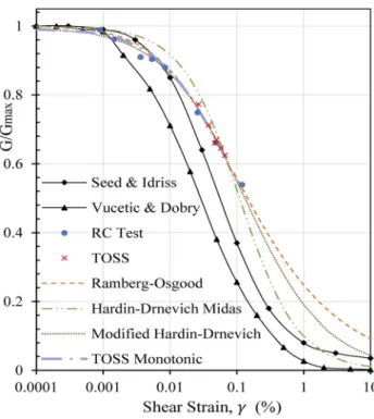
The shear modulus degradation curve can be obtained from the torsional simple shear test, which generates stress-strain hysteresis loops, from which values of the secant shear modulus Gsecare computed with the increasing strain level (Fig. 1).
3. COMBINED RESONANT COLUMN AND TORSIONAL SHEAR TEST
The combined Resonant Column-Torsional Simple Shear Device (RC-TOSS device) related to this study was originally built by Prof Richard Ray at University of Michigan in the 1980s Ray, [9], Ray and Woods, [10]. Then it was rebuilt and calibrated in Gy}or at the Geotechnical Laboratory of the Department of Structural and Geotechnical Engineering at Szechenyi Istvan University for the purpose of the PhD study of Zsolt Szilvagyi in 2013. The testing device was described in detail by Szilvagyi [11] in his thesis.
The tests were conducted on dry sand, a set of resonance column tests in addition to cyclic and irregular tests were
performed up to a stress level of 60 kPa and a confining stress of 94 kPa. For this study, only one irregular TOSS test with a shear stress of 40 kPa was used to evaluate the ability of the material models to predict the dynamic behavior of the soil. An irregular load history was scaled to obtain a maximum value of shear stress of 40 kPa for this stress- controlled TOSS test, and the resulted shear stress-strain curve was used for curve fitting and calibrating the model. In Fig. 2, the maximum shear modulus obtained from RC test is 95,500 kPa, and other RC tests were conducted at higher strains. Shear modulus values from TOSS test were obtained from the monotonic one-way curve, as well as theGsecwhich is the slope of the line that connects the two ends of each of the loops. Figure 2 shows good compatibility between RC and TOSS tests, and also similar behavior to the studies conducted by Seed and Idriss [12] and Vucetic and Dobry [7].
4. MATERIAL MODELS
4.1. Ramberg-Osgood
Ramberg and Osgood [13]first proposed a model with three parameters that would describe the stress-strain curves of aluminum-alloy stainless-steel and carbon-steel sheets. This model wasfirst used in soil modeling by Faccioli et al. [14] to predict the shear modulus degradation curve of sands. The formulation to be used in practical calculations for soils (1) describes the nonlinear stress-strain behavior, and with simple manipulation of the equation, the shear modulus reduction curve (2) and the damping ratio can be obtained as well,
Fig. 1.Estimation of shear modulus during cyclic loading Fig. 2.Shear modulus degradation curves comparison
g¼ τ Gmax
1þa
τ Cτmax
R−1
; (1)
Gsec
Gmax ¼ 1 1þa
Cττmax
R–1 ; (2) wheregis the shear strain,τis the shear stress.Gmaxis the small strain shear modulus, τmax is the maximum shear stress, usually obtained from triaxial test results, and it is a function of the confining stress, angle of friction, and cohesion.a,CandRare curve-fitting constants.
The model was modified to follow the original Masing criteria [15], as the shear modulus for the unloading- reloading curves is equal to Gmax, and the shape of these curves is equal to the one-way curve except that it is enlarged by a factor of 2. Two extra rules have been suggested by Pyke [16] to predict the path of the curves. These rules indicate that the unloading and reloading curves should follow the initial curve in case the previous maximum shear strain is exceeded, and if the current loading or unloading curve intersects a previous one, it should follow the previous curve.
The extended rules can be programmed easily to determine the path that the stress-strain curve will follow for compli- cated load histories. And the original rules can be imple- mented by modifying the one-way equation, as it is shown in Eq. (3),
g ¼ 2
"
ττi
2
Gmax
1þa
ττi
2
Cτmax
R–1!#
þgi; (3) whereτiand giare the shear stress and the shear strain at the turning point respectively.
The modified Ramberg-Osgood model was implemented in Midas GTS code to be used for solid soil layers. However, the equation in Midas shown in Eq. (4) is slightly different than the conventional one,
G0g¼τð1þajτjbÞ; (4) whereG0¼Gmaxand aandbare given by
a¼ 2
grG0 b
; b¼ 2phmax
2phmax ; (5) wherehmaxis the maximum damping constant andgris the reference shear strain.
Extended Masing criteria were also used for the hyster- esis curve
G0
g7g1 2
¼τ7τ1
2
1þa ττ7τ1
2 b
: (6)
4.2. Hardin-Drnevich
Hardin and Drnevich [17] proposed a modified hyperbolic relationship to predict the shear stress-strain behavior of soil. In their study, they found that the stress-strain behavior is not exactly described by a hyperbola. As a result, the hyperbolic equation was modified by distorting the strain
scale to make the real stress-strain curve have a hyperbolic shape. Midas uses the same equation introduced by Hardin and Drnevich given by
τ¼ G0g 1þ
ggr
; (7) whereG0is the initial shear modulus andgris the reference strain, which can be modified to get the best fit with the testing data. Hysteresis curves are formulated on the basis of the Masing’s rule as well
τ¼G0ðgg1Þ 1þ
ðg2ggr1Þ
þτ1: (8)
5. FINITE ELEMENT MODEL IN MIDAS GTS
The model built on Midas for this study is based on the work of Szilvagyi and Ray [18]. However, their paper focused on studying the small strain stiffness of soils, and it verified the capability of the software to model the TOSS test in a more of static manner. Moreover, some modeling difficulties were faced in their analysis, which were fixed in the model developed in this study. This research concentrated mainly on predicting the dynamic behavior of soils under irregular and more complicated loading patterns, which was not captured by the previous study.
Modeling was performed using the cylindrical element coordinate system. The model simulates the TOSS test;
consequently, it consists of a 1 cm thick hollow cylinder with the same dimensions as the tested soil specimen. The mesh elements used in the model are hexahedral of high order;
each element has 20 nodes with the dimensions shown in Fig. 3bin meters.
2017 elements comprise this model, it is pinned at the bottom surface, and all the top nodes are connected with rigid links to a central node which is allowed to move along and rotate around the vertical axis. The prescribed rotation or moment is imposed on this central node, which will simulate the torsional load applied in the TOSS test. No
Fig. 3.Finite element mesh of soil sample, a) elements and nodes, b) dimensions of the middle element
stress irregularities were noticed at the base of the model after the confining stress stage.
The analysis is performed in construction stages in order to simulate the test conditions, where it starts with applying a confining stress of 94 kPa on the free surface of the ele- ments, afterwards, the dynamic material model (R–O or H– D) is set for all the elements, and the torsional loading stage begins. The prescribed rotation around the vertical axis was assigned a time-varying function that is similar to the load history in the TOSS test with a maximum rotation of 0.00338 radians, which will cause an average shear strain in theq-Zdirection of 0.00067 mm/mm. Manual load stepping was not needed before and after turning points, unlike the previous study, and the analysis was stable and converged without problems or high number of iterations.
The method of least squares was used with the help of the solver tool in excel to find the curvature constants values that fit the Ramberg-Osgood (1) and Hardin-Drnevich equations curves with the test data (Table 1), by minimizing the sum of the squares of the strain residuals (the difference between an observed value, and thefitted value provided by a model). The same technique was used subsequently tofind the reference strain that Midas uses in the R–O equation Fig. 4.
6. RESULTS
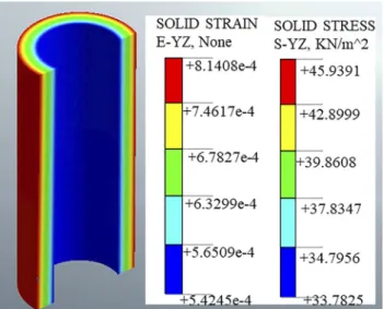
After the first stage, the whole specimen is subjected to a confinement stress of 94 kPa, as a result, the normal solid stresses in the three directions will be the same for all the elements, with no noticeable irregularities even with the pinned bottom surface.
The load history duration is 0.801 seconds, with time increments of 0.001 seconds, which results in 801 total time steps for each analysis. Figure 5 shows the distribution of shear stresses and strains along the radius of the specimen at thefinal increment. As expected, similar observations will be made for both the R–O and H–D soil models, as the dis- tribution is uniform along the height of the specimen and it increases with the distance from the center, which shows the benefit of using a hollow cylindrical specimen for more even distribution of stress and strain along the radius of the sample.
Table 1.Material model parameters used in this study
Parameter Conventional Ramberg-Osgood Midas Ramberg-Osgood Hardin-Drnevich Unit
Initial dynamic shear modulus G0 95,500 95,500 95,500 kPa
Max. shear stress τmax 44.17 – – kPa
Reference shear strain gr 0.000462 0.00148 0.0011 mm/mm
Curvefitting constants a 1 0.0267 – –
C 1.55 – – –
R 1.9 – – –
b – 0.8508 – –
Max. damping constant hmax – 0.19 – %
Dry density gd 17 17 17 kN/m3
Poisson ratio y 0.3 0.3 0.3 –
Fig. 4.Curvefitting for the soil models with the TOSS test data
Fig. 5.Shear stresses and strains distribution along the radius (R–O model), a)q-Zshear stress, b)q-Zshear strain
The average solid stresses and strains in theq-Zdirection (S-YZ, E-YZ) for three elements (inner, middle, and outer elements) in the model were compared to the shear stress- strain curves from the TOSS test for both material models.
Moreover, the dynamic shear modulus was calculated from these curves and compared as well with the shear modulus degradation curves obtained from RC-TOSS tests.
Figure 6shows a very goodfit between the test data and the curves obtained from FEM calculations on Midas using the Ramberg-Osgood model. On the other hand, thefit was not as good when using the Hardin-Drnevich model with the parameters inTable 1as it can be seen inFig. 7, and the calculated values would drift even further from the test data at higher stress levels when using the conventional hyper- bolic Hardin-Drnevich formula (7).
Figure 2 shows how both models predict the shear modulus in the Finite Element Method (FEM) calculations on Midas. The Ramberg-Osgood shear modulus degradation curve was calculated from Eq. (2), which matches perfectly with the FEM R–O calculations in Midas and shows a very good agreement with the RC and TOSS tests. While the modulus reduction curve for the Hardin-Drnevich model, which was obtained from the one-way monotonic curve resulted from analyzing the model on Midas, gives a curve that is higher than the real values until it reaches a strain value of 0.057%, where it drops below the TOSS test curve.
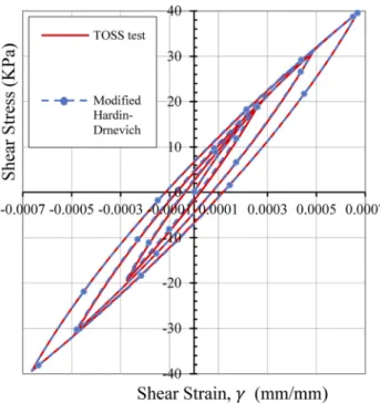
Darendeli [19] suggested modifying the hyperbolic model in order to reach a better representation of the normalized modulus reduction curve by integrating a cur- vature coefficientainto the equation. This modification can be applied to the hyperbolic equation by Hardin and Drnevich for better prediction of the hysteresis behavior of soils. The modified equation is given as follows:
τ¼ G0g 1þ
ggr
a : (9) By using the same method as before (the least square method), the values of the reference strain: gr¼0:00132 mm/mm, and the curvature coefficient: a¼0:7129, give a much better fit with the testing data for both the stress-strain curve (Fig. 8) and the modulus degradation Fig. 6.Shear stress-strain curve from Midas using Ramberg-
Osgood model
Fig. 7.Shear stress-strain curve from Midas using Hardin-Drnevich model
Fig. 8.Modified Hardin-Drnevich model by Darendeli
curve (Fig. 2) than the conventional Hardin-Drnevich model.
7. CONCLUSION
This study concentrates on the dynamic behavior of soils when subjected to irregular loading patterns. Resonant col- umn and TOSS tests were analyzed, and their results were used as a reference to evaluate the ability of the Ramberg- Osgood and Hardin-Drnevich soil models to predict the shear stress-strain curves under such types of loads. The model built on Midas was developed, and some modeling difficulties in the previous model were solved in order for the model to be able to produce accurately more complex hysteretic curves for earthquake load histories. It was confirmed that this model has the capability to imitate the TOSS test conditions, as it shows good agreement with modulus degradation and hysteretic behavior of the soil in the test, especially for the Ramberg-Osgood model, while it was clear that the Hardin-Drnevich model struggled to accurately match the nonlinearity of the shear stress-strain curve. As a result, the curvature coefficient introduced to the equation is suggested to be used by the FEM software for better results. This model can be a useful and convenient tool to simulate the TOSS test for irregular load histories based on a simple cyclic or even one-way test, and then use the parameter for more complex geotechnical problems.
REFERENCES
[1] E. Bak,“Numerical modeling of pile load tests,”Pollack Period., vol. 8, no. 2, pp. 131–140, 2013.
[2] J. Szep,“Modeling laterally loaded piles,”Pollack Period., vol. 8, no. 2, pp. 117–129, 2013.
[3] A. Achouri and M. N. Amrane,“Effect of structures density and tunnel depth on the tunnel-soil-structures dynamical interaction,” Pollack Period., vol. 15, no. 1, pp. 91–102, 2020.
[4] B. Hardin and F. Richart, “Elastic wave velocities in granular soils,”J. Soil Mech. Found. Div.,vol. 89, no. SM1, pp. 33–65, 1963.
[5] B. Hardin and W. Black, “Sand stiffness under various triaxial stresses,”J. Soil Mech. Found. Div.,vol. 92, no. SM2, pp. 27–42, 1966.
[6] T. Wichtmann, M. Navarrete Hernandez, and T. Triantafyllidis,
“On the influence of a non-cohesivefines content on small strain stiffness, modulus degradation and damping of quartz sand,”Soil Dyn. Earthquake Eng., vol. 69, no. 2, pp. 103–114, 2015.
[7] M. Vucetic and R. Dobry, “Effect of soil plasticity on cyclic response,”J. Geotech. Eng. ASCE,vol. 117, no. 89, pp. 89–107, 1991.
[8] K. Ishihara, Soil Behavior in Earthquake Geotechnics. Oxford University Press 1996.
[9] R. P. Ray, “Changes in shear modulus and damping in cohe- sionless soils due to repeated loading,”PhD Thesis, University of Michigan, 1983.
[10] R. Ray and R. Woods,“Modulus and damping due to uniform and variable cyclic loading,”J. Geotech. Eng.,vol. 114, no. 8, pp. 861– 876, 1988.
[11] Z. Szilvagyi, “Dynamic soil properties of Danube sands,” PhD Thesis, Gy}or, Hungary: Szechenyi Istvan University, 2017.
[12] H. Seed and I. Idriss,“Soil moduli and damping factors for dy- namic response analysis,” Technical Report EERC 70-10, Earth- quake Engineering Research Center, University of Cal. Berkeley, 1970.
[13] W. Ramberg and W. R. Osgood, “Description of stress strain curves by three parameters,” Tech. Notes, Natl. Advisory Com- mittee Aeronautics, vol. 902, 1943.
[14] E. Faccioli, V. Santayo, and J. Leone,“Microzonation criteria and seismic response studies for the city of Managua,”inProceedings of Earthquake Engineering Research Institute Conference, San Fransico, California, Nov. 29–30, 1973, 1973, pp. 271–291.
[15] G. Masing,“Self stretching and hardening for brass”(in German), inProc. 2nd Int. Congr. Appl. Mech., Zurich, 1926, 1926, pp. 332– 335.
[16] R. Pyke, “Nonlinear soil models for irregular cyclic loadings,” J. Geotech. Geoenviron. Eng., vol. 106, no. GT11, pp. 715–726, 1979.
[17] B. Hardin and V. Drnevich,“Shear modulus and damping in soils:
Design equations and curves,”J. Soil Mech. Found. Div., vol. 98, no. SM7, pp. 667–692, 1972.
[18] Z. Szilvagyi and R. P. Ray,“Verification of the Ramberg-Osgood material model in Midas GTS NX with the modeling of torsional simple shear tests,”Period. Polytech. Civil Eng., vol. 62, no. 3, pp.
629–635, 2018.
[19] M. B. Darendeli,“Development of a new family of normalized modulus reduction and material damping curves,”PhD Thesis, University of Texas at Austin, USA, 2001.
Open Access. This is an open-access article distributed under the terms of the Creative Commons Attribution 4.0 International License (https://creativecommons.org/
licenses/by/4.0/), which permits unrestricted use, distribution, and reproduction in any medium, provided the original author and source are credited, a link to the CC License is provided, and changes–if any–are indicated. (SID_1)