The role of higher education in spatial mobility

The role of higher education in spatial mobility

Zsolt Tibor Kosztyán^1,2,3* , Vivien Valéria Csányi^1,2, Zsuzsanna Banász^1,2, Ákos Jakobi^3,4,5, Ildikó Neumanné‑Virág^1,3 and András Telcs^1,2,6,7

Introduction

Having knowledge of the migratory behavior of students has been considered extremely important for the relevant institutions and to those who attempt to promote and direct higher education. Certain migratory behavior is determined by socioeconomic and cul- tural features of regions (Lourenço and Sá 2019). Psychologically, those districts where the habitation of certain age group is higher have larger outgoing (Dotti et al. 2013; Telcs et al. 2015) and incoming streams (Beine et al. 2014), as there is a positive correlation between the amount of tutorial services and population. A larger total number of stu- dents (Dotti et al. 2013) tend to be attracted to and held by regions where the unem- ployment is lower and economic opportunities are greater, as the educated workforce often expects to remain in the region (Lourenço and Sá 2019). Kazakis (2019) reports that individuals favor places with lower inequality, housing prices, and taxes. Utility levels and experience factors also play a substantial role in the decision making of pos- sible student settlers (Faggian and Franklin 2014; Franklin and Faggian 2014). On the other hand, living in such densely populated regions is more costly. Beine et al. (2014)

Abstract

The role of higher education in social and spatial mobility has attracted considerable attention. However, there are very few countrywide databases that follow the career paths of graduates from their place of birth, through their enrollment in university, and ultimately to their workplace. However, in Hungary, there is an excellent source maintained by the government’s Education Authority containing information on career tracks, which allows one to follow all students from their place of birth, through their choice of higher education institution, to their workplace. With the combination of gravity‑like economic models and the proposed mobility network, this paper exam‑

ines the mediating and retaining role of institutions. This paper also proposes how to calculate the added value of location and institution in salaries and how to use these values to explain mobility between locations. The paper also shows how economic inequities influence revealed application preferences through the asymmetry of the mobility network.

Keywords: Mobility, Graduate tracking, Temporal and spatial networks, Career tracking system

Open Access

© The Author(s), 2021. Open Access This article is licensed under a Creative Commons Attribution 4.0 International License, which permits use, sharing, adaptation, distribution and reproduction in any medium or format, as long as you give appropriate credit to the original author(s) and the source, provide a link to the Creative Commons licence, and indicate if changes were made. The images or other third party material in this article are included in the article’s Creative Commons licence, unless indicated otherwise in a credit line to the mate‑

rial. If material is not included in the article’s Creative Commons licence and your intended use is not permitted by statutory regulation or exceeds the permitted use, you will need to obtain permission directly from the copyright holder. To view a copy of this licence, visit http://

creat iveco mmons. org/ licen ses/ by/4. 0/.

RESEARCH

*Correspondence:

kzst@gtk.uni‑pannon.hu

1 Department of Quantitative Methods, University of Pannonia, Egyetem str. 10, Veszprém 8200, Hungary Full list of author information is available at the end of the article

finds that language, quality of higher education and university rankings have positive impacts while distance and migration costs have negative impacts on international stu- dent mobility to destination areas. The features and reputations of institutions also play a substantial role. Their quality is often measured by proxies (Lourenço and Sá 2019):

for example, the employability of graduates (Sá et al. 2012; Lourenço and Sá 2019), the teacher-student ratio (Sá et al. 2004), student quality (Dotti et al. 2013), research effec- tiveness (Adkisson and Peach 2008), and the results of international rankings (Ciriaci 2014).

The reported effect of quality differs across studies (Lourenço and Sá 2019). One study reports that there is not enough difference to identify an impact of institutional quality Sá et al. (2012). In other cases, quality seems to matter (Ciriaci 2014; Cooke and Boyle 2011). A recent paper investigates whether research quality is associated with a univer- sity’s ability to attract students from other provinces in Italy. The estimates suggest that research performance is a significant predictor of student enrollment. Cross-country dif- ferences in the quality of higher education institutions (HEIs) may also play a substantial role in international and internal student mobility (Bratti and Verzillo 2019). Mobility decisions depend on the attractiveness of the origin and destination and one’s age and may be justified by emotional or family reasons (Lourenço et  al. 2020). However, the advantages of migration are explored from various perspectives: more interesting teach- ing services, distinct sociocultural skills, and the opportunity to leave one’s home (Hold- sworth 2009; Lourenço et al. 2020). Further research shows a negative effect of distance on students’ mobility decisions (Sá et al. 2004). The direct cost of attending an HEI has received considerable attention in empirical work. Financial support packages, which at least partly cover the expenses of a college education, are available in most higher edu- cation systems. The amount of financial aid, in the form of grants and scholarships, is expected to have a positive effect on the probability of enrollment (Fuller et al. 1982;

Catsiapis 1987). Nevertheless, these financial aid packages rarely cover all out-of-pocket expenses, such that students are often dependent on their families’ financial resources.

Household income is among the most commonly evoked factors when discussing the decision to continue studying after the secondary level, with most studies finding that the higher the income of the household is, the higher the demand for post-secondary education and the propensity to be in school after the secondary level (see, for instance, Savoca 1990; Duchesne and Nonneman 1998; Checchi 2000; Hartog and Diaz-Serrano 2007). Parental educational level and occupational status are sometimes used either to proxy for this income effect or examined in their own right, and they exert a positive influence on young people’s decisions to attend higher education (e.g., Checchi 2000;

Nguyen et al. 2003; Hartog and Diaz-Serrano 2007).

Application to universities (so-called application mobility) is the first step in the spa- tial mobility of young people. The birth-to-school and school-to-work (so-called occu- pation mobility) transitions can be examined using both economic models (see, for instance, Tuckman 1970; Orsuwan and Heck 2009; Niu 2015), such as gravity models (e.g., Agasisti and Dal Bianco 2007; Alm and Winters 2009; Abbott and Silles 2016; Cul- linan and Duggan 2016), and social network analysis (see, e.g., González Canché 2018;

Bilecen et al. 2018; Kondakci et al. 2018).

This study demonstrates advantages of combining economic and data science meth- ods in the analysis of application and occupation mobility. Gadar and Abonyi (2018) analyzed the school-to-work transition in the framework of a bipartite network model using the integrated database of the National Tax Administration, the National Health Insurance Fund, and the Education Authority. Based on the Education Authority data- base, application mobility is investigated using gravity models and logistic regressions (Telcs et al. 2015); however, to the best of our knowledge, no prior work has combined economic and social science methods to analyze the dynamic structure of the mobility network. Combining time-series gravity models and dynamic network science methods allows us to understand changes in the structure of the mobility network. These models can cross-validate one another, and in this way, they can be used for model triangulation (Modell 2015).

Spatial mobility

Spatial or geographical mobility is the movement across different locations. It concerns the physical motion from one space to another (Powell and Finger 2013). It is usually dis- tinguished from social mobility, which is the ability to move up or down in social class (typically defined in terms of wealth). However, sociologists argue that the social mobil- ity of individuals with diverse backgrounds is adversely affected by educational experi- ences (Powell and Finger 2013; Haveman and Smeeding 2006; Brown 2013). Therefore, the spatial mobility of applicants (application mobility) and of graduated early-career people (occupation mobility) are usually motivated by the promise of social advance- ment, such as a better salary, better existence, and better social esteem (Montmarquette et al. 2002; Hilmer and Hilmer 2012). Kazakis (2019) finds a positive and significant rela- tionship between the migration flows of skilled individuals and innovation (patents as proxy), productivity (using, e.g., total factor productivity and labor productivity as prox- ies), higher population density, and higher investments in R&D. He reveals that techno- logical development is highly correlated with education. Highly innovative regions are more attractive to professionals. Grogger and Hanson (2015) analyze how economic and political conditions influence foreign students’decisions to live in the United States after receiving PhDs from US universities. The authors find that students who receive merit- based fellowships or scholarships during their studies and have more educated parents are more likely want to stay in the United States. The authors contend that a stronger US economy makes it more attractive for the graduates to remain in the United States instead of returning to a home country with a weaker economy. Lucas (2001) reveals the factors affecting the international migration of highly skilled people and some benefits of the technology transfers, international trade and capital flows induced by “brain drain”.

Faggian and Franklin (2014) contend that the migration of highly educated persons is fundamental for policy makers. Higher human capital can improve a region’s relative position. They use a negative binomial regression to estimate a gravity-type model of the interstate migration of “college-bound” high school students in the US. Chetty (2020) measure children’s outcomes in adulthood to advance the research on human capital development and find that neighborhoods have causal effects on children’s long-term outcomes.

Despite the divergent results on spatial mobility in the recent social science litera- ture, there are studies examining geographical mobility trends within countries over time (Kulu et al. 2018; Chetty 2020), especially in the case of application and occupation mobility.

Methods for exploring spatial mobility

The diverse methodological approaches for measuring spatial mobility include, on the one hand, direct techniques to quantify the volume of people’s movement in space.

Examples such as traffic counts (Cascetta 1984), population census data (Ette et al. 2008), or commuting surveys (Rüger et al. 2011) rely to varying degrees on concrete measures of the flows between origin and destination; however, the availability of data for such studies is often limited. Another widely used methodological solution is, therefore, the application of indirect tools for exploring geographical mobility. Researchers estimate spatial mobility numbers, for instance, from GPS tracking data (Zheng et al. 2008; Siła- Nowicka et al. 2016; Zignani and Gaito 2010) or cell phone information (Mohall 2015;

Candia et al. 2008; Gonzalez et al. 2008); such methodologies could provide reasonable assumptions on geographical mobility numbers.

Other indirect tools apply proxies, such as distance-based probabilities, to measure the volume of spatial mobility between regions. Rogerson (1990) applied geometric probability methods to estimate migration distances based on the spatial distribution of population and region shape data. It is also common to approximate spatial interactions or mobility volume between regions by taking the size of regions and spatial proximities into account, namely, by applying the gravity model approach from social physics in a geographical context. Moreover, Poot et al. (2016) explicitly highlights the use of gravity modeling in spatial mobility research.

Methodologies related to occupation (or labor) mobility account, for example, for the interaction between the returns to geographic mobility and to the level of education by applying distance functions. Based on a large dataset, Lemistre and Moreau (2009) calculated the distance between the place of education and the location of the first employment of graduated students. Their results suggest decreasing returns to spatial mobility in the distance covered and increasing returns to mobility with higher levels of education. Similarly, Magrini and Lemistre (2013) examine an income-distance trade- off model and found that the most highly skilled young people do not receive a positive wage return from migration but that less-skilled young workers do. Early-career spatial mobility was also analyzed by Venhorst et al. (2015), who applied an instrumental vari- able approach in their model and found positive wage returns related to spatial mobil- ity; however, when controlling for self-selection, a strong reduction was observed in the effect of spatial mobility on job match quality. Similarly, Javakhishvili Larsen and Mitze (2015) applied treatment variables in panel econometric models of individual-based lon- gitudinal data to determine the interconnectedness of spatial mobility and early career effects.

The gravity model

The so-called “gravity” equations are widely used in empirical analysis of foreign trade, migration and even capital flows due to mass-based spatial movements (Anderson

1979). Gravity models have become popular due to their flexibility, simplicity and high explanatory power (excellent fit) Anderson and Van Wincoop (2003). To analyze the spatial interaction between two or more locations using this mathematical model, one applies Newton’s gravitational law, as with gravity in physics (Paas 2003). Countries and municipalities with high economic power exert attraction on smaller ones around them (Nemes Nagy and Tagai 2011). Attractive areas are geographical points (e.g., cit- ies, small regions) where the attractiveness of the place is stronger than that of any other geographical point. Based on the physical analogy, there are two basic areas of applica- tion: the examination of spatial flow (the intensity of the flow) and the delimitation and demarcation of attractive areas (Nemes Nagy and Tagai 2011)

Henri-Guillaume Desart developed a version of the gravity model for analyzing pas- senger travel and applied it to railway planning, and the American economist Henry Carey presented a statement that resembled the notion of a gravity model in 1858 (Odlyzko 2015). According to a survey by Fotheringham et al. (2000), Carey (1858) and Ravenstein (1885) observed that there is a parallel between the movement of individuals between cities and the law of universal attraction, namely, there is a more intense flow between larger cities than between smaller towns (Fotheringham et al. 2000; Ravenstein 1889).

International trade has its own gravity model, developed by Jan Tinbergen (1962). It is a multivariate linear regression model for modeling bilateral and regional trade that is employed for analyzing cross-sectional and panel data (Tinbergen 1962; Anderson 1979). The gravity model of foreign trade, like other gravity models in social science, predicts bilateral trade flows based on the size and distance of the partner economies (Anderson and Van Wincoop 2003). It states that trade between two countries is directly linked to the “gravitational” pull of their national incomes (GDP) and inversely pro- portional to the distance between them (Paas 2003). The model predicts bilateral trade flows based on economic size (usually measured in GDP) and distance (Anderson 1979;

Bergstrand 1985, 1989; Anderson and Van Wincoop 2003). The gravity model has been widely used to estimate the impact of a variety of policy issues, including regional trad- ing groups, currency unions, political blocks, various trade distortions and agreements, border region activities and historical linkages (Paas 2003; Westerlund and Wilhelmsson 2011).

The gravity model also underlies migration studies. Most studies using the gravity model approach have sought to rationalize labor force mobility across locations, espe- cially internal migration waves. There has been highly accurate empirical work on this topic for countries such as the United States (Ashby 2007), China (Shen 1999; Poston and Zhang 2008), Germany (Bierens and Kontuly 2008), Hungary (Cseres-Gergely 2012) and Spain (Devillanova and García-Fontes 1998). Based on the objectives of the present study, the most relevant articles are those examining international migration streams.

In addition to other works, we can also mention articles on international migration to the European Union (Breitenfellner et al. 2008; Warin and Svaton 2008) and to the United States (Karemera et al. 2000) as the two main regions that draw foreign immi- gration. These articles tend to include standard economic variables such as per capita gross domestic product (GDP) or population, sometimes using different changes in var- iables, as in Warin and Svaton (2008), which is based on calculations related to GDP,

while in Karemera et al. (2000), political variables are also included, which has a nega- tive impact on migration flows. The leader countries where most international students are recruited from include China, India and other parts of Asia. Another study finds that “China is becoming an important destination for students due to the distinctive- ness of the language, the rise of its universities in global rankings and the country’s eco- nomic growth” (Ahmad and Shah 2018). According to the gravity model, the number of migrants between two regions is directly proportional to the population in each region and indirectly proportional to the squared distance between the location they leave and the region they enter.

The gravity model approach is also common in higher-education-related spatial mobil- ity studies. Bernela et  al. (2018) tested the significance of the impact of the scientific size of regions and spatial proximity on PhD mobility in France by applying the Heck- man (1979)’s two-step gravity model with a selection equation to evaluate the existence of potential spatial and nonspatial proximity effects. In addition, there are examples of measuring higher-education-related application mobility with large survey-type data- sets. Extensive research on the spatial mobility of graduates was performed by Ven- horst et al. (2011), who applied multinomial logit models to investigate the relationships between migration and both regional economic circumstances and individual character- istics. They found that the presence of a large labor market is the most important struc- tural economic determinant of higher retention rates in regions.

The network model

Mobility can be modeled by networks. In this case, nodes represent locations, while directed arcs represent the mobility from one location to another. The weights of arcs represent the number of domestic migrants (spatial mobility) between given locations.

In network science, null model creation is a common and useful tool. The null model assumes that the network is random (Newman and Girvan 2004) and thus that the weights of the arcs are independent of one another. Liu and Murata (2010)’s null model assumes that the probability of weights on an arc depends on the distance between loca- tions, while Gadár et al. (2018) assumes that the number of links (weights of arcs) fit well to the values predicted by a gravity model. Null models are also essential for modular- ity-based community detection. Modularity-based community analysis is performed in two separate phases: first, the detection of a meaningful community structure from a network and, second, the evaluation of the appropriateness of the detected community structure. Systematic deviations from a random configuration or from other null models without a characteristic modularity structure allow us to define a quantity called mod- ularity, which is a measure of the quality of partitions. Newman and Girvan consider only the degree of nodes as a null model, which is equivalent to rewiring the network while preserving the degree sequence (Newman and Girvan 2004). This random model overlooks the economic nature of the network and thus modules. However, economic- based null models can connect these aspects: modularity-based community detection to find and explain communities where mobility exceeds the expected value. Economic null models predict the weight of arcs and, in this way, establish a baseline and explain network properties such as density, asymmetry or clustering. Therefore, it is worth con- necting gravity and link prediction models. Based on link prediction, other properties of

the network, such as asymmetry, can be evaluated. In this study, we show how to match the network asymmetry and the revealed preference matrix; therefore, the application preference order can also be modeled using economic models.

Most studies on student mobility focus on international movement (see, e.g., Beine et  al. 2014; Shields 2013), and very few studies have investigated mobility within a county (see an excerpt of Bacci and Bertaccini 2020). The reason for the low number of papers in this field is that it is very difficult to access a reliable database containing data on students, employees, and institutions, while several databases on international mobility networks are freely available (Gadár et al. 2020). However, an increasing num- ber of countries, including Italy, Estonia, and Hungary, are registering applicants, and this allows for the investigation of the mobility network. To the best of our knowledge, Hungary is the first in the field of data integration because it has registered applications in a central database since 2001, and since 2011, this database has been integrated into the early career database, which was already an integrated database. In addition, this anonymous database is freely available to researchers.¹

Contribution to the literature

To the best of our knowledge, very few studies have attempted to combine gravity-like and network models (see several exceptions in Gadár et al. 2018; Bacci and Bertaccini 2020). However, they are not combined to explain mobility network formation. Although very few studies still consider economic model-based link prediction, network prop- erties, such as asymmetry, are not modeled by economic inequities, and they are not used to estimate the revealed application preferences. In this study, aspects of describ- ing young people’s mobility are combined (see Fig. 1). The main result of this study is to apply economic gravity models for link prediction, which provides an explanation for why mobility stronger between certain locations. We demonstrate the connection between revealed preferences and network asymmetries, and we show how the revealed application preferences can be explained by economics or rooted in spatial economic inequalities reflected by the gravity-based network asymmetries.

Fig. 1 Combining dynamic network and economic time‑series gravity models

1 http:// dimpl omant ul. hu.

Methods

In section “Data sources”, the common data sources are introduced as indicated in Fig. 1.

Then, in section “Applied null models in mobility networks”, the fundamental network properties are introduced, which will be evaluated for the network based on the eco- nomic gravity model, which is introduced in section “Applied gravity models”. Finally, in section “Methods”, we present the estimates of the inequities in the application prefer- ences through network asymmetry; see section “Modeling application preferences via asymmetries in the application mobility network”.

Data sources

Several specific data sources are involved in the study. One of the main databases is the Hungarian central system for tracking graduates’ careers (HCSTGC). Similar track- ing systems were recently developed by Estonia and Italy (Bacci and Bertaccini 2020;

Kovacs and Kasza 2018). At present, there are few such systems, but we believe that a career path tracking system is the key data source for analyzing student mobility and the impact of higher education on society and the economy. Therefore, it would be worth- while for decision makers to consider introducing such a system at least at the European Union level.

HCSTGC includes anonymized information on the location of residence (NUTS4 sub- region), the city (or subregion) of the HEI, the county and subregion of the workplace, and starting salary of all graduated employees who earned their absolutorium or degree between 09/01/2014 and 01/31/2015. Among these individuals, this study focuses on those who were employed as of May 2016, representing 47,165 graduate students. The occupation and economic activity codes are also available for the work and workplace.

The occupation coding uses the International Standard Classification of Occupations (ISCO) codes. The economic activity coding using the International Standard Indus- trial Classification of all Economic Activities (ISIC) codes. Following Gadar and Abonyi (2018)’s work and databases, the first two letters of the occupation codes are matched to thirteen scientific fields of graduation; we called these fields occupation categories.

The next applied database is the student application database (2006–2017) which contains anonymized data from applicants and HEIs. We used the following data for the analysis: the location (NUTS4 subregion) of the applicant, the location of the HEI, the applied for BA/BSc/MA/MSc program and the scientific field of the program. To maintain consistency between the student application database and HCSTGC, hence- forward, only the thirteen matches for occupation-scientific field category (occupation category) are considered: (1) agriculture, (2) human studies, (3) social sciences, (4) infor- mation technology, (5) law & public administration, (6) military, (7) business & econom- ics, (8) engineering, (9) health & medical sciences, (10) pedagogy, (11) sport sciences, (12) natural sciences, and (13) arts. The aim of the matching was to ensure consistent nomenclature. In this study, only categories of the ISCO are considered, but to ensure consistency, nomenclatures of thirteen scientific fields are used as occupation categories ( O_k,k=1, 2, .., 13).

The last included data sources are already found in all countries in the European Union (such as Eurostat) and most countries in the world. The per-capita gross domestic

income (GDI/cap) of a location (i.e., subregion) between 2006 and 2017 comes from the Hungarian Central Statistical Office. From the Hungarian National Employment Service, we obtained the mean of the (gross) salary² for all 19 counties and the capital city (Buda- pest) for 2015 and 2016. These national (not only for recent graduates) salary statistics are available via ISIC/ISCO codes at the county level.

Applied null models in mobility networks

The mobility network can be described as a directed graph and is an ordered pair G=(V,E) where V is a set of vertices (also called nodes, i.e., locations);

E⊆ {(x,y)|(x,y)∈V²∧x�=y} is a set of edges (also called arcs) that are ordered pairs of distinct vertices (i.e., an edge is associated with two distinct locations in a mobility graph). The number of movements between locations is associated with the edges. E is the adjacency matrix of graph G, where the elements of the matrix indicate whether pairs of vertices are adjacent in the graph.

Denote e_ij as the matrix element of adjacency matrix E of mobility graph G. The first null model that will be considered is the random configuration model that calculates the arc probabilities p^NG_ij , assuming a random graph conditioned to preserve the degree sequence of the original network:

where id represents the in-degree and od the out-degree: idj=

ieij , odi=

jeij , L is the number of arcs (links) between nodes.

The distance-dependent (Liu and Murata 2010) version can also be used for null models.

where p^α,β is the distant-dependent null model. f(d_ij) is a monotone function of dis- tance decay. The α,β parameters are called importance values estimated by regression analysis.

For the economic model we use the notation q_ij^Ŵ=p^α,β,δ_ij with multiindex Ŵ= {α,β,δ}

where m_i is an economic value, such as GDP, GDI or another economic quantity of the location of node i. d_ij is the distance between location i and location j. α,β,δ are importance values of locations and the distance between locations. They were estimated through a regression analysis. In this study, we propose a generalized gravity model for link prediction (null model):

(1) p^NG_ij = idiodj

L

(2) p^α,β_i,j = od_i^αid_j^β

f(d_ij)

(3) q^Ŵ_ij =γd_ij^δm^α_im^β_j

2 There is a flat tax of 33.5% in Hungary.

where N is the number of economic parameters while α_k,β_k,γ,δ are regression parameters.

The time-series version of the null model predicts the arcs of the dynamic network.

Null models are mainly used in modularity-based community analysis. Originally, the method was specified for edges.

In the case of a directed network, this difference can be formulated as follows:

pij represents the number of estimated arcs/weights proceeding from the i-th to the j-th location, and δ

C_i,C_j

is the Kronecker delta function that is equal to one if the i-th and j-th locations are assigned to the same community.

The goal of modularity-based community analysis is to separate the network into groups of nodes that have fewer connections between them than inside communities (Newman and Girvan 2004). The modularity of partition C can be calculated as the sum of the modularities of the C_c,c=1,. . .,n_c communities:

Originally, these null models were specified for estimating arcs in a binary graph; how- ever, they have been extended to handle weighted graphs, but null models can also be used to evaluate asymmetry.

The value of modularity Mc of a cluster Cc can be positive, negative or zero. Should it be equal to zero, then the community has as many links as the null model predicts.

When modularity is positive, the C_c subgraph tends to be a community that exhibits a stronger degree of internal cohesion than the model predicts.

To obtain real communities, null models (p in Eq. (10) ) should approximate a given property ( ), such as the probability of arcs, weights, reciprocity or edge asymme- try as much as possible. Therefore, when seeking null models, the following equation should be minimized:

(4) q^Ŵ_ij =γd_ij^δ

N

k:=1

m^α_i^k

km^β_j^k

k

(5) log(q_ij^Ŵ)=log(γ )+δlog(d_ij)+

N

k:=1

α_klog(m_ik)+β_klog(m_jk)

(6) log(q_t,ij^Ŵ )=log(γ )+δlog(d_ij)+

N

k:=1

α_klog(m_t,ik)+β_klog(m_t,jk)

f(C) = (fraction of arcs within communities)− (7)

− (null model based expected fraction of such arcs) .

f(C)= 1 (8) L

i,j

e_ij−p_ij δ

C_i,C_j

M_c= 1 (9) L

(i,j)∈Cc

(e_ij−p_ij).

where is the modeled parameter, such as the arc/weights between node i and node j or the asymmetry of arc ij.

Measuring asymmetry: We consider a directed weighted network specified by the (nonnegative) weight matrix E , where e_ij indicates the weight of the directed from node i to node j. In the case of no connection from i to j, e_ij=0 . E can be specified as the sum of a symmetric ( P ) and skewed symmetric matrix Q , where

The edge asymmetry matrix ( A ) is the rate of skew-symmetric ( Q ) and symmetric ( P ) components of the weight matrix ( W).

where aij = ^e_e^ij−eji

ij+eji ∈A is also a skewed symmetric matrix. For ∀ i = j, where ei,j+ej,i �=0 , edge asymmetry can only be interpreted for the interconnected i and j nodes. It satisfies that −1≤a_ij= −a_ji≥=1 — in binary networks a_ij ∈ {−1, 0, 1}.

The economic null model for asymmetry (denoted as ) can be expressed as follows:

Equation (15) also shows that while the economic version of the law of gravity is distance dependent (see Eq. (3)), by substituting it into Eq. (14), we obtain a distance-independ- ent model. In addition, the economic null model of asymmetry only depends on the eco- nomic parameters (denoted as m) of locations and their importance factors ( α,β ). The indicator ^Ŵ

i,j has economic content itself. If q_i,j^Ŵ estimates domestic immigration and q_j,i^Ŵ estimates domestic emigration between location i and location j, then q_i,j^Ŵ-q^Ŵ_j,i represents the net mobility exchange while q^Ŵ_i,j+q_j,i^Ŵ represents the gross mobility exchange between location i and location j. If the arcs represent import/export goods, then the absolute value of ^Ŵ

i,j is a well-known intraindustry trade (IIT), while in this study, this value is called the intramobility rate (IMR), which characterizes the asymmetry of the mobility between locations.

Applied gravity models

According to the introduced data sources (see "The gravity model" section) we can iden- tify and calculate the following parameters and coefficients (see Table 1):

(10)

ij

|_ij−pij| =ǫ→min

(11) E=(P+Q)

(12) P=1

2

E+E^T

(13) Q=1

2

E−E^T

(14) A= Q

P, aij = e_ij−e_ji e_ij+e_ji ∈A

(15) ^Ŵ_ij = q^Ŵ_ij −q^Ŵ_ji

q^Ŵ_ij +p^Ŵ_ji = γd_ij^δm^α_im^β_j −γd_ij^δm^α_jm^β_i

γd_ij^δm^α_im^β_j +γd_ij^δm^α_jm^β_i = m^α_im^β_j −m^α_jm^β_i m^α_im^β_j +m^α_jm^β_i

Table 1 Notations and explanations Notation Explanation

Lj Location (subregion at the NUTS level 4) Lj indexed by j C(Lj) County of location Lj.

Ok Occupation Ok (coded by ISCO) indexed by k.

Yi,j Number of movements from location Li to location Lj.

Yi,j|k Number of movements from location Li to location Lj , restricted only to the occupation Ok. HEIm Higher education institution (HEI) m, indexed by m.

HEI(Lj) 1, if there is an HEI at location Lj . 0, otherwise.

HEIj|k 1, if there is an HEI that has a program for the expectation of occupation Ok. Lm Location (subregion at the NUTS level 4) of HEIm

RANKm,t Faculty excellence rank of HEIm in year t (based on Eduline domestic HEI rank).

Ai,j,t Number of applications from location Li to HEIj in year t

Am,m^′,t The number applications where HEIm is ahead of HEI_m^′ on the preference list in year t

Ij=GDI/cap(Lj) Per‑capita gross domestic income of location Lj , and Im will be used for GDI/cap at the location of HEIm.

URj=UR(Lj) Unemployment rate of location Lj. En Employee En , indexed by n

S_k,j,m^g (n) Starting salary of a graduated employee En working in occupation Ok at location Lj and gradu‑

ated in HEIm.

Sⁿ_k Mean (starting) salary of undergraduate or not graduated employees in occupation Ok. S^g_k Mean (starting) salary of graduated employees in occupation Ok.

S^g_k,j Mean (starting) salary of graduated employees in occupation Ok at location Lj

S^g_k,j,m Mean (starting) salary of graduated employees in occupation Ok at location Lj , graduated from HEIm.

Fig. 2 An illustrative example of the added value of education and location to starting salary

The added value measured by the salary premium, which is the difference between the starting and mean salary of not graduated employees, can be specified by a sum of a graduate premium, the added value of the location, added value of the HEI and indi- vidual wage bargaining (see the waterfall plot in Fig. 2).

Figure 2 shows that the added value of a location can be negative; however, except for the mean salary of undergraduates, every factor can either be positive or negative (Table 2).

Factors of starting salary: After matching education-occupation pairs and the calcula- tion of average salaries, the following differences can be specified:

Formally, the starting salary for employee n can be explained as follows (see Eq. (16)):

where ǫ_n is the result of individual wage bargaining. Figure 2 explains how the salary pre- mium ( S_k,j,m^g (n)−S_k,j,m ) for employee n can be divided into four parts, namely, the graduate premium ( S^g_k ), the added value of the location ( S^g_k,j ), the added value of the HEI ( S^g_k,j,m ), and the individual bargaining ( ǫ_n ) as described in Eq. (16).

These values serving as proxies for the added value to salaries will be measured, and they will be applied as dependent variables in the proposed spatiotemporal model.

Two kinds of movement can be specified based on the Hungarian career tracking database: (1) application to an HEI (see the solid arrows in Fig. 3a) and (2) application to a job (see the dotted arrows in Fig. 3a). These movements can be separated (see Fig. 3b) into two distinct layers. Two kinds of mobility, occupation mobility ( Y_Li,Lj ) and application mobility ( A_Li,HEIj,t ), can be explored. In addition, based on the appli- cation databases, application mobility can be modeled over the period 2006–2017 with a fixed effects gravity model. Occupation mobility is also separated in time (see Fig. 3b). One of the problems is that these movements differ over time. Therefore, it (16) S^g_k,j,m(n)−S_k,j,m=�S^g_k+�S^g_k,j+�S^g_k,j,m+ǫ_n

Table 2 Income differences and their meaning

Differences Meaning

S^g_k=S^g_k−Sⁿ_k Graduate premium

S^g_k,j = S^gk,j−S^g_k Added value of the location

S^g_k,j,m = =S^g_k,j,m−S^g_k,j The added value of HEI ( HEIm ) at

location ( Lj ) for occupation ( Ok).

Fig. 3 Spatiotemporal networks for modeling both birth‑to‑school and the school‑to‑work mobility

is a so-called two-layer spatiotemporal network. Nevertheless, if we only consider the movement between the location of residence before the application to an HEI and the location of a workplace, we can propose a so-called mobility network (see Fig. 3c). In this case, the edges between nodes connect different locations not only in space but also in time.

There are two ways to understand the proposed mobility network. We can regard the mobility network as a spatiotemporal mobility network where the communities repre- sent the “attractiveness” of a location. The sizes of communities can differ, regardless of whether an HEIs is present. Counties that typically represent sources and sinks for different occupations can be specified. The role of an HEI in becoming a source or sink county can also be analyzed.

The other understanding is to regard mobility as a flow (of people) between locations.

Gravity models make it possible to model the “attractiveness” of a location, such as the strength of the regional economy (GDP/cap, GDI/cap), salary opportunities, the distance dependencies between locations for every single occupation, and the role of institutions.

The logarithmic form of the proposed spatiotemporal gravity model can be specified as follows for occupation mobility:

where u_j,j^′ is the residue of the regression model. β s are the regression parameters to be estimated. Note that the years of the data values Ij,tj =GDI/cap(Lj,tj) and I_j^′_,t^′

j =GDI/cap(L^′_j,t_j^′) are usually different. When considering the source location ( L_j ), the GDI/cap(L_j,t_j) should be from the year of application, while when considering the target ( L^′_j ) (workplace), the GDI/cap(L^′_j,t_j^′) should be from the year of hiring at the workplace.

Using dummy variables, the role of HEIs is included in Eq. (17). GDI/cap values are proxies for the expected salaries; therefore, if the salary surplus (as an added value) of the location for an occupation O_k is considered, then a detailed model can be specified as follows:

Application mobility can be explored with a time-series (fixed effects gravity) model. In this way, similar indicators can be specified.

(17) logY_j,j^� =𝛽₀+ 𝛽₁logI_j,tj+ 𝛽₂logI_j^�_,t^�

j+

+ 𝛽₃logUR_j,t

i+ 𝛽₄logUR_j�,t_j^�+ 𝛽₅logd_j,j�+

+ 𝛽₆HEI(L_j) + 𝛽₇HEI(L_j�) +u_j,j�

(18) logY_j,j^�|_k =𝛽₀+ 𝛽₁logS^g_k,j+ 𝛽₂logS^g_k,j� + 𝛽₃logUR_j,tj+

+ 𝛽₄logUR_j^�_,t^�

j + 𝛽₅logd_j,j^� + 𝛽₆HEI_j|_k+ 𝛽₇HEI_j^�|_k+

+u_j,j^�|_k

(19) logA_j,m,t =𝛽₀+𝛽₁logI_j,t+𝛽₂logI_m,t+

+𝛽₃logUR_m,t+𝛽₄logUR_j,t+𝛽₅logd_j,m+ +𝛽₆RANK_m,t+u_j,m,t

We linked the gravity models (Eqs. (17)–(19)) and the linked prediction models (see Eqs.

(5)–(6)).

Owing to the time-series data, the application mobility can be explored using time- series (i.e., fixed effects gravity) models. Therefore, the dynamic null model predicts the dynamic mobility graph.

Table 3 reports which null models are estimated with economic models.

Modeling application preferences via asymmetries in the application mobility network The Hungarian Education Authority has made all application data available to research- ers. We considered the interval between 2006 and 2017. According to (Telcs et al. 2016), individual application preferences can be aggregated, and in this way, professional, regional, and institutional aggregated preference matrices can be calculated. Here, an (i, j) cell from the aggregated preference matrix shows how many times the i-th insti- tution preceded the j-th institution in student applications. Telcs et al. (2016) offered several heuristic methods to estimate aggregated preference orders from an aggregated preference matrix. They showed that these methods approximate the optimal preference order very well, where the optimal preference order is a preference order and the num- ber of opposite application preferences (i.e., the sum of values in the lower triangle of the Table 3 Connections between null models and economic gravity models

Network Static or dynamic Null model Economic model

Occupation mobility network Static Equation (5) Equations. (17)–(18)

Application mobility network Dynamic Equation (6) Equation (19)

Preference graph Dynamic Equation (15) Equation (20)

Table 4 The unordered aggregated preference and asymmetry matrices

V I1 I2 I3 I4

(a) Preference matrix

I1 0.0 1.0 2.0 3,0

I2 2.0 0.0 2.0 3,0

I3 1.0 1.0 0.0 3,0

I4 0.0 0.0 0.0 0,0

3.0 2.0 4.0 9.0

N^o 2 1 3 4

Opposite preferences=2+1+1=4

A I1 I2 I3 I4

(b) Asymmetry matrix

I1 0,0 −1/3 1/3 1,0

I2 1/3 0,0 1/3 1,0

I3 −1/3 −1/3 0,0 1.0

I4 −1.0 −1.0 −1.0 0.0

−1.0 −5/3 1/3 3.0

N^o 2 1 3 4

Sum of the lower triangular=−10/3

preference matrix) is minimal (Telcs et al. 2016). One possible choice is the column sum method.

The aggregated revealed preference is the order of the column sums (see Table 4a).

Since Eq. (14) is a monotonous transformation, the order of the column sum is not mod- ified (see Table 4b), the asymmetry is not perturbed, and therefore, we gain a model for the preference order (see Eq. (20)).

Table 4 provides an example of an (unordered) aggregated preference matrix.

Telcs et al. (2016) showed that if the matrix is (re)ordered by the preference orders, then the opposite preferences (the sum of the values in the lower triangle) can be decreased. The algorithm will stop if the (re)orderings of the preference matrix cannot reduce the sum of opposite preferences (see Table 5).

Equation (20) shows an example of the power of combining economic models and net- work science. Equation (20) explains the preference value between institutions HEI_m and HEI_m^′ in year t. If these models fit well, then the institutional preference order can also be modeled and explained.

Equation 20 defines the asymmetry between HEIs m and m^′ . A generalized gravity model is used to express the attractiveness of the HEIs to express the asymmetry of the nodes in the network representing the HEIs.

For shorter notation here, we used I_m instead of GDI/cap(L_HEIm) with a little abuse of the original notation.

(20) A_m,m^′_,t= I_m^α1UR^αm²RANK_j^α3−I_m^β1′UR^β_m²′RANK_m^β3′

I_m^α1UR^α_m²RANK_m^α3+I_m^β1′UR^β_m²′RANK_m^β3′

Table 5 The ordered aggregated preference and asymmetry matrices

V I2 I1 I3 I4

(a) Preference matrix

I2 0.0 2.0 2.0 3,0

I1 1.0 0.0 2.0 3,0

I3 1.0 1.0 0.0 3,0

I4 0.0 0.0 0.0 0,0

2.0 3.0 4.0 9.0

N^o 1 2 3 4

Opposite preferences (E)=1+1+1=3

A I2 I1 I3 I4

(b) Asymmetry matrix

I2 0,0 1/3 1/3 1,0

I1 −1/3 0,0 1/3 1,0

I3 −1/3 −1/3 0,0 1.0

I4 −1.0 −1.0 −1.0 0.0

−5/3 −1.0 1/3 3.0

N^o 1 2 3 4

Sum of the lower triangular=−4

Results

In this section, we show how the location and the location’s economic state influence the students mobility, career path and how it can be inferred by our models.

Added value of the locations and education

Following Eq. (16), the salary premium can be decomposed into four components. The first is the graduate premium S^g_k , which is the difference between the mean start- ing salary of graduated employees ( S^g_k ) and the mean starting salary of not graduated employees

(Sⁿ_k ) in occupation category k. Figure 4 shows the graduate premiums by occupation category k. The highest mean salaries are in information technology, engineering and business & economics. The highest added value of a master’s diploma is also in these three categories.

The second factor is the added value of the location. Figure 5 shows the added value of the location for business & economics (see Fig. 5a) and engineering (see Fig. 5b).

The added value, which can be positive or negative, is ordered into ten deciles. In the case of business and economics, only the seventh decile contains positive values, and these deciles are concentrated in the center of Hungary, while in the case of engineering,

0 300 600 900 1,200 1,500

Arts Natural Sciences Sport Sciences Pedagogy Health & Medical Sciences Engineering Business & Economics Military Law & Public Administration Information TechnologySocial Sciences Human Studies Agriculture

Not grad.

BA/BSc MA/MSc

Fig. 4 Graduate premiums (EUR/month) by occupation category

Fig. 5 Added value of locations to salaries (10 deciles)

added value is concentrated in the western part of the country. These results are highly correlated with the spatial distributions of the companies. While the center of econom- ics is concentrated in the capital city, the companies requiring engineers are concen- trated in the more industrialized western part of Hungary.

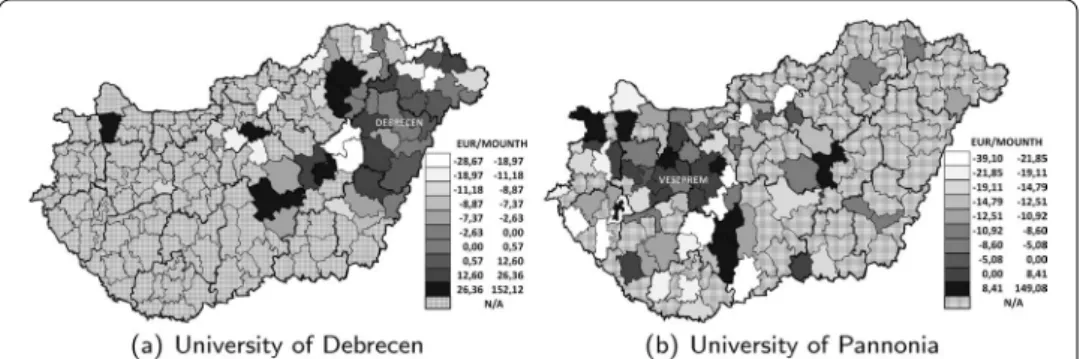
The third factor is the added value of HEIs. The role of HEIs in spatial mobility has already been shown in Fig. 6. If an employee graduated in the eastern part of Hungary (i.e., the University of Debrecen, see Fig. 6a) then he/she usually does not go to work in to another part of the country, and vice versa. For example if employees graduated in the western part of the country, for example from the University of Pannonia (see Fig. 6b), which has several campuses in the western part of Hungary, then they usually do not work in the eastern part of the country. The added value of rural universities is positive or neutral in the locations and neighboring locations of the campuses; however, it is usually negative in the capital (Budapest) and varies substantially in more distant subregions.

The remaining factor is the individual bargaining on salary, which is the unex- plained (residual) part of the economic model in Eq. (16). This value follows the normal distribution.

Analyzing spatial mobility to reflect the role of HEIs

In this section, application and occupation mobility are investigated. First, traditional gravity models are applied to determine the roles of economic and institutional indica- tors of mobility. Then, a mobility network is built and the main network properties are examined. In the null models, parameters, such as link weights, density and asymmetry, are predicted by the unified economic-network model. Then, the preference orders of institutes and subregions are explained by the proposed economic-network model.

Analyzing application mobility: the first step

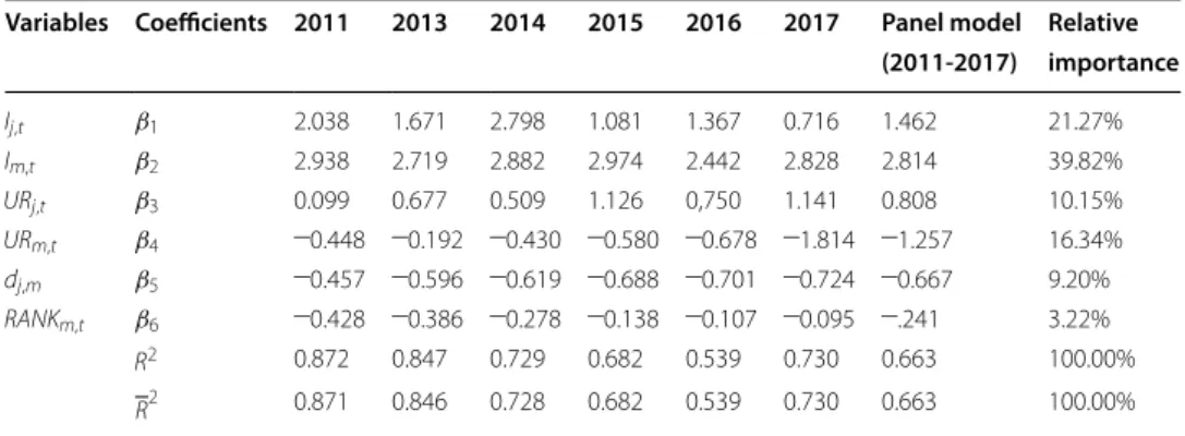
Applying gravity models: With Eq. (19), the primary preferences can be analyzed within the period 2011–2017. We used a fixed effects gravity model. Table 6 shows the results.

I=GDI/cap is only a proxy for the cost of living and expected salaries. It is not sur- prising that the most important value is the GDI/cap in the subregion of the HEI. Nev- ertheless, the second most important value is the GDI/cap in the subregion of residence

Fig. 6 Added value of the HEIs to salaries (10 deciles) in business & economics

of the applicants, which indicates that the economic properties of the sending subregion also play an important role in being accepted by an HEI.

The unemployment rate (UR) of the subregion of the place of residence has a posi- tive effect while the unemployment rate of the subregion of the university has a nega- tive effect on applications. This means that there are more applicants from subregions with higher unemployment rates but that fewer apply to institutions in subregions where this indicator is also high. In the national ranking of Hungarian HEIs, the bet- ter HEIs are linked to fewer applicants; therefore, having a negative value indicates that more reputable institutions enroll students.

Note that the role of institutional reputation is decreasing each year. The negative coefficient of distance is also in line with the gravity models. The larger the distance is, the higher the travel costs, resulting in a greater financial burden for parents and students. In addition, between 2011 and 2016, this coefficient linked to physical dis- tance increased, which indicates a decrease in mobility since the geographical dis- tances did not change.

Telcs et  al. (2015) suggested that gravity models should be used without HEIs in capital cities because the high centralization of institutes may distort the results.

The gravity-based potential model shows that the role of Budapest (BP) is increas- ing. The strength of Budapest-centric HEIs is reflected in the greater difference in potential values between Budapest and rural HEIs (see Fig. 7).

Applying network science models: Network analysis can not only confirm the results of the gravity model but also offers additional insights. One of the fundamental dynamic network indicators is the change in network density over time (see Fig. 8a) and the change in the structure of modules (see Fig. 8b). Figure 8a shows that between 2011 and 2013, the density of the mobility graphs was almost equal regardless of whether one includes of excludes the HEIs in Budapest. The linear trends show that the density is increasing, which indicates that fewer locations are connected. Furthermore, not only has the number of applicants decreased, but students have applied to HEIs from fewer locations. The differences in the slope of the linear trend indicate that the decrease in mobility is greater if HEIs in Budapest are excluded. In 2017, there were 27% fewer appli- cants to HEIs than in 2011. This causes the lines to be thinner in Fig. 8b. The module- based community analysis identified similar catchment areas as the potential analysis.

Table 6 Results of the gravity model for all first‑place applications to higher education institutions (2011–2017)

Variables Coefficients 2011 2013 2014 2015 2016 2017 Panel model Relative (2011-2017) importance

Ij,t β1 2.038 1.671 2.798 1.081 1.367 0.716 1.462 21.27%

Im,t β2 2.938 2.719 2.882 2.974 2.442 2.828 2.814 39.82%

URj,t β3 0.099 0.677 0.509 1.126 0,750 1.141 0.808 10.15%

URm,t β4 −0.448 −0.192 −0.430 −0.580 −0.678 −1.814 −1.257 16.34%

dj,m β5 −0.457 −0.596 −0.619 −0.688 −0.701 −0.724 −0.667 9.20%

RANKm,t β6 −0.428 −0.386 −0.278 −0.138 −0.107 −0.095 −.241 3.22%

R² 0.872 0.847 0.729 0.682 0.539 0.730 0.663 100.00%

R² 0.871 0.846 0.728 0.682 0.539 0.730 0.663 100.00%

However, it indicates that the Eastern part is more fragmented. In addition, the decreas- ing density (with the exception of 2016) indicates that fewer students applied to HEIs and that they applied from fewer places.

The results of the fixed panel model show the increasing roles of the distance between the subregion of the student’s residence and the subregion of the HEI (see Table 6). The higher values of the distance deterrence function at low distances in 2017 also reflect these results; nevertheless, the distance deterrence function shows the nature of the distance distribution between the student’s residences and the loca- tions of HEIs. The maximum of all deterrence functions is in the low distance between locations, which indicates the retention role of HEIs. In both curves, a fraction can be seen showing that students are welcome to apply to institutions in the center of the

Fig. 7 Results of the gravity‑based potential models (2011, 2017). BP: Budapest, the capital of Hungary

Fig. 8 Densities and modules in the dynamic application network (2011–2017). *The density is the number of edges between subregions of students’ residence and theHEI/(number of HEIs number of subregions).

**The thickness of the edges is proportional to the number of applications; outward linesindicate loops