APPLICATIONS OF COMPUTER VISION: SKYLINE EXTRACTION AND CONGRESSIONAL DISTRICTING

(1)

APPLICATIONS OF COMPUTER VISION: SKYLINE EXTRACTION AND

CONGRESSIONAL DISTRICTING

Ph.D. Thesis

Balázs Nagy

Doctoral School of Economics, Business and Informatics

Supervisor: Attila Tasnádi, D.Sc.

Department of Mathematics

Institute of Mathematics and Statistical Modelling Corvinus University of Budapest

Budapest, 2020

(2)

(3)

Acknowledgements

Throughout the writing of this thesis, I have received a great deal of support and assistance.

I would like to thank my supervisor, Attila Tasnádi, for his dedicated support and guidance. He has continuously provided encouragement and always been supportive and enthusiastic from my undergraduate studies to the doctoral thesis. I have also learned a lot from István Deák about the practical aspects of research.

I would like to express my deepest gratitude to my colleagues, friends, and family.

I cannot possibly thank my parents, my sister, and my brother enough for their support. Finally, I am deeply thankful to my wife.

(4)

List of Tables

2.1 Results of automatic skyline extraction method. . . 24 2.2 Experimental results of the eld tests. . . 28

(7)

List of Figures

2.1 AR application for mountain peak identication. Source: Author. . . 11

2.2 The determination of the panoramic skyline. Source: Author. . . 15

2.3 The extraction of the skyline. Source: Author. . . 18

2.4 Connected components labeling. Source: Author. . . 21

2.5 Matching of the panoramic skyline with the extracted skyline. Source: Author. . . 22

2.6 Some examples of automatic skyline extraction. Source: Author. . . . 26

2.7 Field test images with the extracted skyline, the panoramic skyline, and the reference object. Source: Author. . . 27

3.1 The layout of the districts. Source: Author. . . 38

3.2 Example of pack and crack principle. Source: Author. . . 43

3.3 Another example of pack and crack principle. Source: Author. . . 44

4.1 The C_β curve and the comparison of M with the classical circularity indexes on two dissimilar shapes. Source: Author. . . 56

4.2 The computation of the new measureM. Source: Author. . . 58

4.3 Comparison the circularity of two districts by C_β. Source: Author. . . 59

4.4 Arkansas's3^rddistrict in the107^thand1^stdistrict in the113^thCongress. Source: Author. . . 59

(8)

4.5 Iowa's 1^st district in the 107^th and 2^nd district in the 108^th Congress.

Source: Author. . . 60 4.6 The C_β curve and the comparison of M with the classical circularity

indexes on Arkansas's 2^nd district in the113^th and Illinois's4^th district in the 107^th Congress. . . 61 4.7 The boundaries of the 113^th Congress. Arkansas, Iowa, Kansas and

Utah are highlighted. Source: Author. . . 62 4.8 The congressional of Arkansas districts for the 107^th, 108^th and the

113^th US Congresses. Source: Author. . . 63 4.9 The congressional districts of Iowa for the 107^th, 108^th and the 113^th

US Congresses. Source: Author. . . 64 4.10 The congressional districts of Kansas for the107^th,108^thand the113^th

US Congresses. Source: Author. . . 64 4.11 The congressional districts of Utah for the 107^th, 108^th and the 113^th

US Congresses. Source: Author. . . 65 4.12 The evaluation of Arkansas's 3^rd district in the 107^th, 108^th and 113^th

US Congresses by M and the classical circularity indexes. Source:

Author. . . 66 A.1 Example for skyline extraction. Source: Author. . . 73 A.2 Example for skyline extraction. Source: Flickr Creative Commons. . . 74 A.3 Example for skyline extraction. Source: Flickr Creative Commons. . . 75 A.4 Example for skyline extraction. Source: Author. . . 76 B.1 The circularity indexes of Arkansas for the 107^th, 108^th and the 113^th

US Congresses from top to bottom. Source: Author. . . 79 B.2 The circularity indexes of Iowa for the 107^th, 108^th and the 113^th US

Congresses from top to bottom. Source: Author. . . 82

(9)

B.3 The circularity indexes of Kansas for the107^th,108^thand the113^th US Congresses from top to bottom. Source: Author. . . 84 B.4 The circularity indexes of Utah for the 107^th, 108^th and the 113^th US

Congresses from top to bottom. Source: Author. . . 86

(10)

List of Abbreviations

AR Augmented Reality 2, 813, 25, 26

DEM Digital Elevation Model 811, 1315, 20, 22, 23, 63 DMC Digital Magnetic Compass 8, 9, 23, 24

EXIF Exchangeable Image File Format 22 FoV Field of View 12

GIS Geographic Information System 25

GNSS Global Navigation Satellite System 9, 13, 14, 22, 26 HFoV Horizontal Field of View 18, 19, 22

IR Infrared 13

LSI Lee-Sallee Index 49, 55, 57, 59 PPT Polsby-Popper Test 49, 55, 57, 59 RT Reock Test 49, 55, 57, 59

UAV Unmanned Aerial Vehicle 11, 13 VR Virtual Reality 10

(11)

Chapter 1 Introduction

Computer vision is an interdisciplinary eld of science that tries to imitate the ability of humans how they detect and interpret visual data from the environment. Accord- ing to a story, computer vision started as a student summer project at MIT in 1966.

Marvin Minsky asked his undergraduate student Gerald Jay Sussman to link a computer to a camera to describe what it saw. However, this problem is eortlessly done by humans, it proved to be more complicated for computers endowed with algorithms.

As Szeliski noted in 2011 [67], despite all of the advances, the aim for a computer to interpret an image at the same level as a two-year-old is a dream. Nevertheless, this discipline has developed tremendously in the last years. Nowadays, computer vision is applied in many areas, for instance, robotics, industrial automation, trac control, navigation, medical imaging, and surveillance.

Interestingly, techniques that are developed in computer vision could be applied in social sciences as well. For example, the shape of electoral districts might be the subject of visual analysis. Drawing new electoral district boundaries or, in other words redistricting is always a controversial process since it may favor a specic party in an electoral system. Unfortunately, gerrymandering is a commonly used practice of political manipulation that dates back to 1812 when Elbridge Gerry, the governor

(12)

of Massachusetts, approved a redrawing plan of electoral districts that contained a district that reminded journalists of a salamander. This story also explains the origin of this term. Nowadays, gerrymandering is still a hot issue in the United States, where redistricting is often carried out to resolve geographic malapportionment caused by demographic changes. In fact, only a few states have an independent body in charge of this process because state legislatures usually have primary control over redistricting in their state.

Intending to connect the two seemingly distant elds, in both cases, we try to imitate humans as they percept and interpret the environment. On the one hand, matching the visible paramount peaks and landmarks around us with a large-scale map is a traditional way of orientation in mountainous terrain. On the other hand, the visual inspection of the compactness of a congressional district by an outline map is a natural way to look for political manipulation.

Our rst goal is to develop an algorithm for skyline extraction, calculating the azimuth in mountainous terrain, and verify the method in a relevant environment. Our next aim is to prove that optimal partisan districting and majority securing districting are NP-complete problems, and demonstrate why nding optimal districting in real-life is challenging, as well. Finally, we intend to create a parameter-free circularity measure that can be used to detect gerrymandering and apply it to congressional districts. In this dissertation, we also study a computer vision problem and political districting problems, where Part I and Part II contain our results, respectively.

In Chapter 2, we show an eective method that can improve orientation by using skyline in an Augmented Reality (AR) mobile application. These apps, e.g., PeakVisor [62], PeakFinder [65] have a well-developed mountain identication function. They can render the digital terrain model and labels the name of peaks nearby and additional information. Some apps can also annotate uploaded pictures but the

(13)

horizontal orientation is usually imprecise, so manual ne-tuning is required for an appropriate result. It is well known that these apps have a serious problem with the accuracy of the azimuth angle provided by the sensors of the device. The fusion of the digital magnetic compass, accelerometer, and gyroscope gives the translation and rotation of the observer in the 3D space. However, the precision is usually not appropriate since the compass is prone to interference when using it near metal objects or electric currents. With the camera and a digital elevation model, a calibration can be carried out to determine the correct orientation angles. Skyline extraction is a challenging task because various visibility and weather conditions might occur. We propose an eective method to adjust the azimuth by skyline extraction that does not require manual interaction. Chapter 2 is based on Nagy [7].

In Part II, we turn to the analysis of the political districting problems and gerrymandering, which have great importance to society.

In Chapter 3, we study the districting problem from a theoretical point of view.

In the middle of the previous century, it was hoped that the problem of gerrymandering could be overcome by computer programs using only data on the geographic distribution of the voters without any statistical information on voters' preferences and thus determining an unbiased districting, see Vickery [72]. The computational diculty of the problem was clear from the very beginning, see Nagel [47]. The rst algorithm nding all districtings with equally sized, connected, and compact districts was given by Garnkel and Nemhauser [28]. Altman [2] showed that the problems of achieving any of the three mentioned criteria are NP-hard. Moreover, he also demonstrated that maximizing the number of competitive districts is also NP-hard. We show that optimal partisan districting and majority securing districting in the plane with geographical constraints are NP-complete problems. We provide a polynomial time algorithm for determining an optimal partisan districting for a simplied version

(14)

of the problem. Besides, we give possible explanations for why nding an optimal partisan districting for real-life problems cannot be guaranteed. Chapter 3 contains our results published in Fleiner et al. [26].

In Chapter 4 demonstrates an empirical study on gerrymandering. Shape analysis has special importance in the detection of manipulated redistricting. Thus we apply image moments that are widely used in image processing and computer vision. These moments are invariant to similarity transformations and can be calculated eectively.

The eort to create as compact districts as possible can naturally be expected, and it is a standard criterion, see Webster [73], Polsby and Popper [54]. Hence, measuring the circularity of districts can be a suitable tool to help detect gerrymandering. The standard meaning of circularity is the degree to which a shape diers from a circle, and it is the most important index from a practical point of view. A desirable shape circularity measure should be applicable on every planar shape, ranges from 0 to 1, and it should be invariant with respect to translations, rotations, and scaling.

We introduce a novel circularity measure based on Hu moment invariants. We also analyze the shape of Arkansas, Iowa, Kansas, and Utah after redistricting through multiple US Congresses. Chapter 4 is based on Nagy and Szakál [10] and [9].

Finally, in Chapter 5, a brief conclusion summarizes the thesis and presents the contributions.

(15)

(16)

Part I

SKYLINE EXTRACTION

(17)

(18)

Chapter 2 Improving the Azimuth in Mountainous Terrian

An AR application has a serious problem with the accuracy of the azimuth provided by mobile devices. The azimuth (ϕ) is an angular measurement between a reference direction and true north, and a line from the observer to the point of interest, projected on the same plane. The fusion of the Digital Magnetic Compass (DMC), accelerometer, and gyroscope gives the translation and rotation of the observer in 3D space. Unfortunately, the precision is not always appropriate since DMC is prone to interference when using it near metal objects or electric currents, which causes a problem in everyday use. The silhouette of ridges separates the sky from the terrain and forms the skyline or sometimes referred to as the horizon line in a mountain scenery.

This salient feature can be used for orientation in both the traditional paper map way and digitally. With the camera of the device and a Digital Elevation Model (DEM), the correct azimuth can be determined. The skyline extraction from an image is a challenging task because various visibility and weather conditions might occur. We propose an eective method to adjust the azimuth by recognizing the skyline from an image and matching it with the panoramic skyline of the DEM. This algorithm

(19)

does not require manual interaction, and it has also been validated in a real-world environment.

Computer vision algorithms aim to perceive and interpret visual data coming from the environment by describing it and reconstructing its principal properties.

The typical steps of a computer vision task are image acquisition, image processing, feature extraction, and decision making. There are several elds where computer vision is applied, e.g., robotics, industrial automation, transportation, navigation, medical imaging, and surveillance. Humans interpret the environment by processing information that is contained in visible light radiated, reected, or transmitted by the surrounding objects. Due to the larger and higher resolution mobile screens, smart devices have become suitable for navigation since they are equipped with necessary sensors, such as Global Navigation Satellite System (GNSS), DMC, accelerometer and gyroscope. The GNSS and the magnetic eld of Earth give a rough estimate of the position of the observer, but the accuracy of mobile sensors is not high enough for high precision AR applications. The compass is biased by metal and electric instruments nearby, although frequent calibration, so measuring the magnetic and thus the true north is not reliable. The location of the magnetic poles does not coincide with the geographic poles. Moreover, the magnetic poles are wandering around. So, the magnetic north should be corrected using a declination angle to obtain true north. Several studies, for example Blum et al. [13], Höltz et al. [31]

have examined sensor reliability in real-world tests and showed the error of DMC could be as high as 10−30^◦. The error of the gyroscope and accelerometer are also increasing with the elapsed time, and the accuracy of GNSS could be up to several meters. However, these problems are not that critical from our perspective.

Visual orientation is a three-dimensional problem of nding the orientation (pan, tilt, roll) from a geotagged photo. This task requires that the position (longitude,

(20)

latitude, elevation) of the observer is at least roughly given, the photo is taken not far from the ground, and the camera is approximately horizontal. That means the problem can be reduced to a one-dimensional instance in which the pan angle or, in other words, the azimuth needs to be determined. In this case, the camera helps to increase the precision of the other sensors by capturing visual clues whose real-world positions are known from a digital map. We propose a real-time method that extracts skyline from an image and matches it with the panoramic skyline determined from a rendered DEM. Thus, the orientation of the observer can be improved, which is critical in AR applications.

A potential application of visual orientation is mobile hiking apps that annotate mountain photos by matching images with 3D terrain models and geographic data.

The ideal hiking app should have the following features: rendered 3D terrain models, highly detailed spatial data, and AR mode with automatic orientation. Popular AR apps such as PeakVisor and PeakFinder have a well-developed mountain identication function. These apps render the digital terrain model and label the name of peaks nearby with additional information. Some apps can also annotate oine geotagged images. The main problem with these programs that the horizontal orientation is usually imprecise, so a manual correction is required for an appropriate result. One of the few applications that employs sophisticated algorithms is PeakLens [53], but it focuses solely on this function. The fully panoramic360^◦ version of this app by La Salandra et al. [63] can be used with Virtual Reality (VR) devices too. Lütjens et al. [44] give a good example of how VR can oer intuitive 3D terrain visualization of geographical data.

Our main contribution is a novel edge-based method for automatic skyline extraction and a real-time procedure that increases the accuracy of the azimuth. This algorithm could be a module in a future AR app, as it is demonstrated in Figure 2.1.

(21)

(a) Camera picture.

(b) DEM with geographical data.

(c) AR overlay.

Figure 2.1: AR application for mountain peak identication. Source: Author.

(22)

A camera picture is shown in Figure 2.1a with a mountain ridge in the background.

Figure 2.1b introduces the DEM with pertinent geographical data such as trails and peaks. The fusion of the original image and the main hiking data can be seen in Figure 2.1c.

In recent years there has been considerable interest in the challenging task of visual localization in mountainous terrain. In realistic scenarios, vegetation changes rapidly as well as lighting and weather conditions. Since the most steady and reliable feature is the contour of the mountains, people usually use the skyline and the prominent features of a landscape for orientation. This is the main idea in our approach.

Many experts have examined the so-called drop-o problem when the observer or an Unmanned Aerial Vehicle (UAV) is dropped o into an unfamiliar environment and try to locate its position. Preliminary work by Stein and Medioni [66] focused on pre-computed panoramic skyline matching with manually extracted skylines. Tzeng et al. [70] investigated a user-aided visual localization method in the desert using DEMs. Once the user marked the skyline in the query image manually, this feature was looked up in the database of panoramic skylines that had been rendered from a DEM. Camera pose and orientation estimation from an image and a DEM were studied by Naval et al. [49]. This non-real-time approach classied the sky and non- sky pixels by a previously trained neural network. Peaks and peak-like protrusions were used as feature points in the matching phase, where pre-calculated synthetic skylines were stored in a database which is not favorable in a real-time AR app due to the computation and storage needs.

Fedorov et al. [24] proposed a framework for an outdoor AR application for mountain peak detection called SnowWatch, and also described the data manage- ment approach of their solution. Sensor inaccuracy and position alignment were only partially discussed. In contrary to the present study, they took in input the device

(23)

orientation, as well. Eventually, they reached a slightly higher peak position error (1.32^◦) on their manually annotated dataset. SwissPeaks is another AR app that overlays peaks is presented by Karpischek et al. [36]. The main limitation of the app is that the correct azimuth should be set manually since visual feature extraction or matching was not implemented. Lie et al. [42] examined skyline extraction by a dynamic programming algorithm that looked for the shortest path on the edge map based on the assumption that the shortest path between image boundaries is the skyline. A similar solution was investigated by Hung et al. [33], where a support vector machine was trained for classifying skyline and non-skyline edge segments. A comparison of four autonomous skyline segmentation techniques that use machine learning was reviewed by Ahmad et al. [1]. The above-mentioned studies focused on skyline extraction only, and their outcomes are hard to compare with our results.

A non-real-time procedure for visual localization was suggested by Saurer et al.

[64]. They introduced an approach for large-scale visual localization by extracting skyline from query images and using a collection of pre-generated, vector-quantized panoramic skylines that were determined at regular grid positions. For sky segmentation, they used dynamic programming, but their solution required manual interaction by the operator in case of the problematic pictures, which amounted to 40% of the samples. An early attempt was made by Behringer [12] to use computer vision methods for improving orientation precision. Due to computation complexity, this solution was tested in a non-real-time environment. Baboud et al. [5] also presented an automatic, but non-real-time solution for annotation and augmentation of mountainous photos. From geographical coordinates and camera Field of View (FoV), this system automatically determined the pose of the camera relative to the terrain model by using contours extracted from the 3D model. They used an edge-based algorithm for skyline detection and proposed a metric for ne-matching based on the feasible

(24)

topology of silhouette-maps. However, their algorithm was well-developed, but it is not suitable for AR applications. An unsupervised method for peak identication in geotagged photos is examined by Fedorov et al. [25]. They extracted the panoramic skyline by edge detection from the rendered DEM, but they did not address exactly how to obtain the skyline from an image.

It is worth to note that Infrared (IR) cameras were also put in an application for localization in a mountain area by Woo et al. [74]. They designed a procedure for UAV navigation based on peak extraction. Special sensors that are sensitive in the IR range could work better under lousy weather or weak light conditions. Unfortunately, a real-world test was not presented in their study.

Visual localization in an urban environment is a related problem. Several studies have been carried out on visual-aided localization and navigation in cities where the sky region is more homogeneous than other parts of the image. For instance, Ramalingam et al. [57] employed skyline, and 3D city models for geolocalization in GNSS challenged urban canyons. Zhu et al. [76] matched the panoramic skyline extracted from a 3D city model with a partial skyline form an image.

This chapter is organized as follows: Section 2.1 describes the proposed method that has three main phases:

1. panoramic skyline determination from DEM, 2. skyline extraction from the image,

3. matching the two skylines.

Section 2.2 presents the experimental results and the eld test. Finally, conclusions and outlook are drawn in Section 2.3.

(25)

(a) Position of the observer in DEM. (b) Panoramic skyline on a satellite image.

(c) Coordinate transformation.

0 90 180 270 360

Azimuth (°) -15

0 15 30

Elevation angle (°)

(d) Panoramic skyline vector.

Figure 2.2: The determination of the panoramic skyline. Source: Author.

(26)

2.1 Method

We propose a method that consists of three main phases. Firstly, we determine the panoramic skyline from the DEM by a geometric transformation based on the idea that Zhu et al. [76] suggested. After that, we extract the skyline from the image by a novel edge-based algorithm that uses connected component labeling. Finally, for the matching phase, we seek the largest correlation between the two skyline vectors.

C++ and OpenSceneGraph were used for panoramic skyline determination. The image processing task and matching were carried out by MATLAB (Image Processing Toolbox). The georeferencing for the eld tests was made with Google Earth Pro and QGIS.

2.1.1 Panoramic Skyline Determination

Panoramic skyline is a vector obtained from the 3D model of the terrain. We used publicly available DEMs: SRTM [23] and ASTER [48], sampled at a spatial resolution between 30m and 90m. Depending on the distance of the viewpoint from the target and characteristic of the terrain in the corresponding geographical area that could be a bit coarse, but in most cases, this resolution was enough. Figure 2.2 demonstrates this phase. Figure 2.2a shows a rendered DEM, where the black triangle is the position of the camera, which was determined by the GNSS sensor of the device. The 360^◦ panoramic skyline was calculated from this point by a coordinate transformation, as Figure 2.2c shows, where

C(X₀, Y₀, Z₀) is the position of the camera,

D(X, Y, Z)is an arbitrary point of the DEM,

D⁰(x⁰, y⁰, z⁰) is the projection of point D. ¹

1y⁰ =Y₀

(27)

Hereby, each point can be described by the azimuth angle:

ϕ=











0 if X =X₀ and Z =Z₀

arcsin z⁰−Z0

ρ

if X ≥X0

−arcsin

z⁰−Z0

ρ

+π if X < X₀ and the elevation angle:

θ= arcsin

Y −y⁰ r

where

ρ=p

(x⁰−X₀)²+ (z⁰−Z₀)² is the distance between C and D⁰ and

r =p

(X−X₀)² + (Y −Y₀)²+ (Z−Z₀)²

is the distance between C and D. A 3D to 2D transformation was applied since the height information, or the radial distance is no longer required. Azimuth angleφand the elevation angle θ describe any point D in the DEM. Finally, the largest θ value determines the demanded point of the skyline for each ϕ. Figure 2.2b illustrates the panoramic skyline projected on a satellite image. The sharp edges on the left corner indicate the border of the DEM because the skyline was calculated only at a reasonable distance. Figure 2.2d shows the output, i.e., the panoramic skyline vector that will be used in the matching phase.

2.1.2 Skyline Extraction

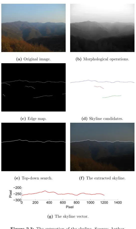
The skyline sharply demarcates terrain from the sky on a landscape photo. Our novel and automatic skyline extraction method is presented in the following. The main idea is based on the experience that large and wide connected components in the upper region of the image usually belong to the skyline.

(28)

(a) Original image. (b) Morphological operations.

(c) Edge map. (d) Skyline candidates.

(e) Top-down search. (f) The extracted skyline.

(g) The skyline vector.

Figure 2.3: The extraction of the skyline. Source: Author.

(29)

A well-known algorithm for connected components labeling was used for nding blobs in a binary image. It is an algorithmic application of graph theory, where connected components are labeled uniquely. Figure 2.4a shows an input binary image with disjoint edge segments that are colored to dierent shades of gray in the output, as Figure 2.4b shows. A ood-ll algorithm was applied for nding 8-connected components (8-connected neighborhood), where pixels touch one of their edges or corners, i.e., they are connected horizontally, vertically, or diagonally. A detailed review of connected components labeling is found in He et al. [29]. It is not necessary to detect the whole skyline since, in most cases, recognizing only an essential part of it is enough for matching. On the other hand, it is crucial to extract a piece from the real skyline and not a false edge. Statistically speaking, the False Acceptance Rate (Type II error) should be as low as possible, while the False Rejection Rate (Type I error) is not that critical.

In the preprocessing phase, morphological operations were carried out to enhance the grayscale image and remove noise. Morphological closing (dilation and erosion) eliminate small holes, while morphological opening (erosion and dilation) removes small objects from the foreground that are smaller than the structuring element. A disk-shaped structuring element was used either for closing and opening but with a dierent radius (5 and 10 pixels). Details on morphology can be found in, e.g., Szeliski [67].

The following algorithm selects the skyline from skyline candidates in multiple steps. The candidates were sorted by the function

S(C) =µ(C) + 2ρ(C),

where C is a skyline candidate, µ measures the number of pixels in the candidate and ρis the span of the candidate, i.e., the dierence between the rightmost and the leftmost pixel coordinates in the image space.

(30)

This function takes into account the size and the span of C with double weight, which is proved to be ecient according to our observations. Therefore, larger and broader skyline candidates are preferred.

The main steps are listed below and also shown in Figure 2.3.

1. Preprocessing

(a) The rst step is to resize the original image to 640×480 pixels and adjust the contrast. (Figure 2.3a)

(b) The sky is in the sharpest contrast to the terrain in the blue color channel in RGB color space. Thus we use the blue channel as a grayscale picture.

(c) Morphological closing and opening operations are applied for smoothing the outlines, reducing noise, and thereby ignoring the useless details, e.g., edges of tree branches or rocks. (Figure 2.3b)

(d) The edge detection is carried out by the Canny edge detector [15] results in a bitmap that contains the most distinctive edges on the image. (Figure 2.3c)

2. Connected components labeling detects the connected pixels on the edge map determining the skyline candidates. The top three skyline candidates are chosen by the function S. (Figure 2.3d)

3. A top-down search selects the rst edge pixels from the most probable candidates in each column because the skyline should be on the upper region of the image. (Figure 2.3e)

4. In case of low resolution, the top-down search might make a one-pixel gap in the skyline. A so-called bridge operation repairs this problem by lling the holes.

(31)

5. The second connected component analysis eliminates the left-over pieces from the edge map and selects the largest one as the presumed skyline. (Figure 2.3f) 6. Finally, the skyline is vectorized for the matching phase. (Figure 2.3g)

(a) Binary image. (b) Three disjoint components.

Figure 2.4: Connected components labeling. Source: Author.

2.1.3 Skyline Matching

The last phase of the proposed method is matching the panoramic skyline and the recognized fragment of the skyline from the image. We look for the point from where the skyline vectors interlock, i.e., the image skyline ts into the panoramic skyline.

Theϕcould be obtained from here. It is worth noting that for the proper comparison, the Horizontal Field of View (HFoV) of the camera and the panoramic skyline² need to be synchronized via the sampling rate of the two signals. For the sake of simplicity, the rst index of the panoramic skyline vector corresponds to 0^◦ (true north) as a reference point. In the case of partially extracted image skyline, the gap also should be considered in accordance with HFoV, so the total width of the skyline is estimated.

After that, normalized cross-correlation(a ? b)is used, which is commonly used in signal processing as a measure of similarity between a vector a (panoramic skyline) and shifted (lagged) copies of a vectorb (extracted skyline) as a function of the lagk.

2The HFOV of the panoramic skyline is 360^◦.

(32)

After calculating the cross-correlation between the two vectors, the maximum of the cross-correlation function indicates the point K where the signals are best aligned:

K = argmax

0^◦≤k<360^◦

((a ? b)(k)).

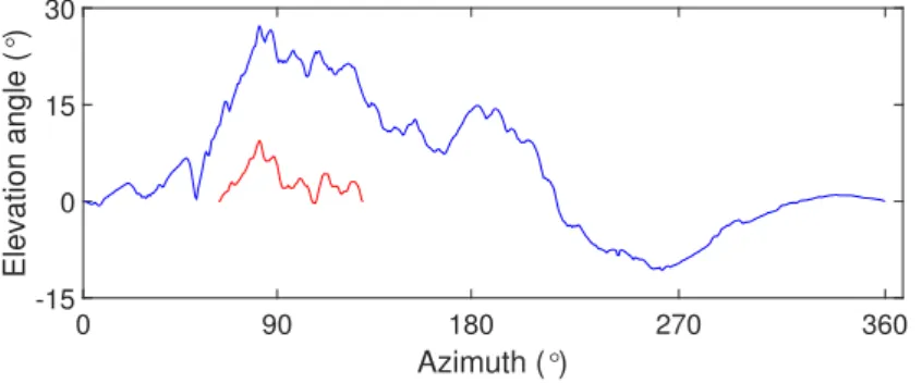
From K the azimuth ϕ can be determined, and the estimated horizontal orientation can be acquired. As it was mentioned above, the camera is supposed to be approximately horizontal when the picture was taken, though the skyline could be slightly slanted. The cross-correlation is not sensitive to such inaccuracies, so this approach is suitable for matching the skylines. An example of matching the panoramic skyline (blue) with the extracted skyline (red) is presented in Figure 2.5.

0 90 180 270 360

Azimuth (°) -15

0 15 30

Elevation angle (°)

Figure 2.5: Matching of the panoramic skyline with the extracted skyline. Source:

Author.

2.2 Experimental Results

Our goal was to develop a procedure that can determine the exact orientation of the observer in a mountainous environment by a geotagged camera picture and a DEM.

The main contribution of this paper was an edge-based skyline extraction method.

Thus the rst part of this section demonstrates the results on sample images. The second part is about calculating the azimuth (ϕ) and comparing the results with

(33)

the ground truth azimuth (ϕˆ) determined by traditional cartographic methods using reference objects.

2.2.1 Skyline Extraction

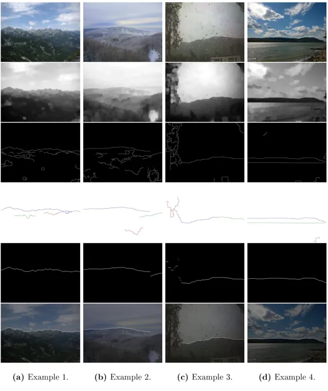
Skyline extraction is a crucial task in this method. The whole pattern is not necessarily needed for the correct alignment because, in most cases, only a characteristic part of the skyline is enough for matching. The algorithm was tested on a sample set that contains mountain photos from various locations, seasons, under dierent weather and light conditions. The goal was to extract the skyline as precisely as possible, therefore to somehow evaluate the results, we also classied the outputs. The pictures were made by the author, or they were downloaded from Flickr under the appropriate Creative Commons license. The collection consists of 150 images with 640×480 pixels resolutions and 24-bit color depth. Experiments showed that this resolution provides good results considering computation performance, as well. Fig- ure 2.6 illustrates the automatic skyline extraction steps on four dierent examples:

(a) shows a craggy mountain ridge with clouds and rocks that could have misled an edge detector; in (b) the snowy hills blend into the cloudy sky mountain which makes skyline detection dicult; (c) is taken from behind a blurry window, where raindrops and occluding tree branches could have impeded the operation of an algorithm; (d) demonstrates a hard contrast image with a clear skyline, where clouds might have induced false skyline edges. The detailed description of the steps can be found in Section 2.1. For more examples, see Appendix A.

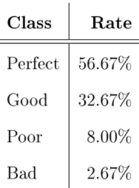
The outputs were classied into four classes according to the quality (%) of the result. The evaluation was done manually because an objective measure is hard to create.

Perfect: the whole skyline [95 −100%] is detected, no interfering fragments

(34)

Class Rate Perfect 56.67%

Good 32.67%

Poor 8.00%

Bad 2.67%

Table 2.1: Results of automatic skyline extraction method.

found.

Good: the better part of the skyline[50−95%)is detected, false pixels do not aect the analyses.

Poor: only a small part of the skyline [5−50%) is detected, false pixels might aect the analyses.

Bad: skyline cannot be found or the detected edges do not belong to the skyline [0−5%).

Table 2.1 shows that the extracted skylines are assigned to Perfect or Good classes in more than89% of the samples. In these cases, the extracted features can be used for matching in the next phase. It is noteworthy that the rate of poor is8% and bad outcomes is less than3%. When the algorithm fails, the diculties usually arise from occlusion, foggy weather, or low light conditions. In some cases, when the picture is hard contrast with plenty of edges, e.g., deceptive clouds, or rocks, the largest connected component did not necessarily belong to the skyline, and it is dicult to nd the horizon line even with the naked eye.

(35)

2.2.2 Field Tests

Unfortunately, it was not possible to compare the results directly with those obtained by other methods discussed above, due to the dierent problems they addressed.

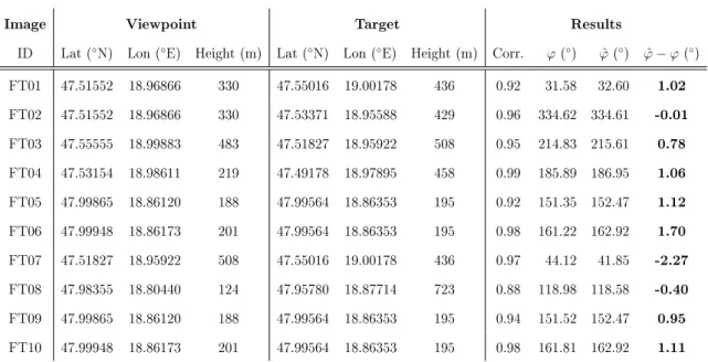
Therefore, we made eld tests to measure the performance of our algorithm. The experiments aimed to determine the orientation using only a geotagged photo and the DEM. A Microsoft Surface 3 tablet was employed, which has an in-built GNSS sensor and an 8MP camera sensor with 53.5^◦ HFoV. Various pictures were taken in the mountains with clearly identiable targets such as church or transmission towers and aligned them into the center of the image with the help of an overlying grid. The Exchangeable Image File Format (EXIF) data contains the position, so a recognizable target concerning the viewpoint could be manually referred, soϕˆwas determined for the10sample images. The low sample size is due to the dicult task of locating test points and the lack of a publicly available image data set with georeferenced objects.

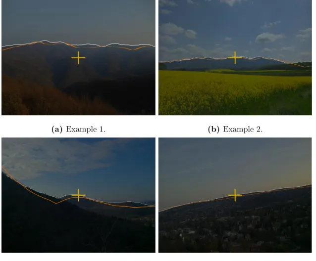
Figure 2.7 shows example images with the extracted skyline (white), the panoramic skyline (orange), and the reference object (yellow cross) that was aligned to the center of the picture. Table 2.2 presents the experimental results of the eld tests. Only Good and Perfect skylines were accepted for the tests, and the correlation is almost 95% on average. The mean of absolute dierences between ϕˆ and ϕ is 1.04^◦, which is auspicious.

As it was mentioned above, the error of DMC could be 10−30^◦. Measuring the inaccuracy of the compass sensor is beyond the scope of this study. Nevertheless, this problem was experienced during eld tests. The benet of the proposed algorithm is the precise orientation obtained by the camera picture and a DEM. The eld tests demonstrated that it could be achieved with this method. The average 1.04^◦ error is mainly caused by the coarse resolution of DEMs and the vegetation. Thus, the results might be enhanced with a higher resolution DEM.

(36)

(a) Example 1. (b) Example 2. (c) Example 3. (d) Example 4.

Figure 2.6: Some examples of automatic skyline extraction. Source: Author.

2.3 Concluding Remarks

This chapter proposed an automatic method for improving the azimuth measured by the unreliable DMC sensor in mountainous terrain. The aim was to develop an algo-

(37)

(a) Example 1. (b) Example 2.

(c) Example 3. (d) Example 4.

Figure 2.7: Field test images with the extracted skyline, the panoramic skyline, and the reference object. Source: Author.

rithm for an outdoor AR app that overlays useful information about the environment from a Geographic Information System (GIS) such as peak names, heights, or distances. The main contribution of this work is the robust skyline extraction procedure that employed connected components labeling. The skyline was extracted successfully in more than 89% of the sample set. Furthermore, eld tests were also carried out to verify the skyline matching, as well. The deviation of the azimuth provided by the algorithm and the ground truth azimuth is 1.04^◦ on average. Performance issues were beyond the scope of this study, but the algorithm is time and storage ef-

(38)

Image Viewpoint Target Results

ID Lat (^◦N) Lon (^◦E) Height (m) Lat (^◦N) Lon (^◦E) Height (m) Corr. ϕ(^◦) ϕˆ(^◦) ϕˆ−ϕ(^◦) FT01 47.51552 18.96866 330 47.55016 19.00178 436 0.92 31.58 32.60 1.02 FT02 47.51552 18.96866 330 47.53371 18.95588 429 0.96 334.62 334.61 -0.01 FT03 47.55555 18.99883 483 47.51827 18.95922 508 0.95 214.83 215.61 0.78 FT04 47.53154 18.98611 219 47.49178 18.97895 458 0.99 185.89 186.95 1.06 FT05 47.99865 18.86120 188 47.99564 18.86353 195 0.92 151.35 152.47 1.12 FT06 47.99948 18.86173 201 47.99564 18.86353 195 0.98 161.22 162.92 1.70 FT07 47.51827 18.95922 508 47.55016 19.00178 436 0.97 44.12 41.85 -2.27 FT08 47.98355 18.80440 124 47.95780 18.87714 723 0.88 118.98 118.58 -0.40 FT09 47.99865 18.86120 188 47.99564 18.86353 195 0.94 151.52 152.47 0.95 FT10 47.99948 18.86173 201 47.99564 18.86353 195 0.98 161.81 162.92 1.11

Table 2.2: Experimental results of the eld tests.

cient. The results are promising, and they showed that the proposed method could be applied as an autonomous, highly accurate orientation module in a real-time AR application. With suitable data and some adaptation, the system might be used for visual localization in GNSS challenged urban environment.

(39)

Part II

CONGRESSIONAL DISTRICTING

(40)

(41)

Chapter 3 Optimal Partisan Districting on Planar Geographies

In this chapter, we examine districting in a particular framework from a theoretical point of view. We show that optimal partisan districting and majority securing districting in the plane with geographical constraints are NP-complete problems.

Furthermore, we provide a polynomial time algorithm for determining an optimal partisan districting for a simplied version of the problem. Besides, we give possible explanations for why nding an optimal partisan districting for real-life problems cannot be guaranteed.

In electoral systems with single-member districts or even with at least two multi- member districts, redistricting has to be carried out to resolve geographic malapportionment caused by migration and dierent district population growth rates. An inherent diculty associated with redistricting is that it may favor a party. The problem becomes even worse if redistricting is manipulated for an electoral advan- tage, which is referred to as gerrymandering.

In the middle of the previous century, it was hoped that the problem of gerrymandering could be overcome by computer programs using only data on voters' ge-

(42)

ographic distribution without any statistical information on voters' preferences and thus determining an unbiased districting, see Vickery [72]. The rst algorithm nding all districtings with equally sized, connected, and compact districts was given by Garnkel and Nemhauser [28]. Earlier Hess et al. [30] provided an algorithm striving for similar goals. However, their algorithm did not always obtain optimal solutions. The computational diculty of the problem was clear from the very beginning. Nagel [47] documented in an early survey the computational limitations of automated redistricting by considering the available programs of his time. Altman [2] showed that the problems of achieving any of the three mentioned criteria are NP-hard. Moreover, he also demonstrated that maximizing the number of competitive districts is also NP-hard. Because of the computational diculty of the problem there is a growing literature on new approaches to nding unbiased districtings, see, for instance, Mehrotra [46], Bozkaya et al. [14], Bacao et al. [6], Chou and Li [19], Ricca [61], Ricca et al. [60]. For recent surveys, we refer to Ricca et al. [59], Tasnádi [69], Kalcsics [35].

Though nding an equally sized districting is already computationally hard, from another point of view it is feared by the public that the continuously increasing computational power makes the problem of carrying out optimal partisan gerrymandering possible. However, the underlying diculty of the problem does not allow us to determine an optimal partisan redistricting. Indeed, Altman and McDonald [3] provide recent evidence that current computer programs are far away from nding optimal gerrymandering.

A formal proof establishing that a simplied version of the optimal gerrymandering problem is NP-complete was given by Puppe and Tasnádi [56]. They took geographical constraints into account, but planarity was not prescribed explicitly. In recent work, Lewenberg et al. [41] also proved the NP-completeness of optimal ger-

(43)

rymandering in the plane. However, they did not demand equally or almost equally sized districts.

This chapter is organized as follows. In Section 3.1, we introduce the most important denitions. In Section 3.2, we show that winning an election, i.e., deciding the existence of a districting that guarantees a majority of a party is also NP-complete.

Furthermore, for districting problems that can be simplied to a one-dimensional districting problems, we provide a polynomial time algorithm for nding the optimal partisan districting. In Section 3.3, we bring forward arguments in favor of the computational intractability of determining an optimal partisan districting for real-life problems of modest size. Finally, conclusions are drawn in Section 3.4.

3.1 The Framework

We assume that parties A and B compete in an electoral system consisting only of single member districts. A single member district is an electoral district returning only one representative to an oce. In addition, voters with known party preferences are located in the plane and have to be divided into a given number of almost equally sized districts. The districting problem is dened by the following structure:

Denition 3.1.1. A districting problem is given by Π = (X, N,(xi)i∈N, v, K,D), where

X is a bounded and strictly connected¹ subset of R²,

the nite set of voters is denoted by N ={1, . . . , n},

the distinct locations of voters are given by x₁, . . . , x_n∈int(X),

the voters' party preferences are given v :N → {A, B},

1We call a bounded subsetAofR²strictly connected if its boundary∂Ais a closed Jordan curve.

(44)

the set of district labels is denoted by K ={1, . . . , k}, where bn/kc ≥3, and

D denotes the nite set of admissible districts consisting of bounded and strictly connected subsets of X and each of them containing the location of bn/kc or dn/ke voters,² and furthermore,

we shall assume that based on their locations then voters can be partitioned into k districts {D₁, . . . , D_k} ⊆ D.

Observe that in dening the districting problem, we assumed that obtaining an almost equally sized districting is possible, which can be justied by the fact that nding an admissible districting for real-life problems is possible, while nding a districting satisfying additional requirements such as partisan optimality is dicult.

In particular, the sta hired to produce a districting map could always construct a districting map consisting of almost equally sized districts, although other properties like partisan optimality are dicult to prove or to confute. Producing a districting with almost equally sized districts is a tractable problem if there are not too many geographical restrictions since then we can obtain a result by drawing districts from left to right and from top to bottom on a map of a state by keeping the average district size in mind. An initial step for such an algorithm would be, for instance, to order the voters increasingly according to their horizontal or vertical coordinates.

We shall mention that in reality, the basic units of a districting problem from which districts have to be created are census blocks or electoral wards rather than voters in order to simplify the problem, and at the same time to include natural municipal boundaries. In this case, voter preferences v : N → {A, B} have to be replaced by a function of type v⁰ : N⁰ → [0,1], where N⁰ stands for the nite set of wards, assigning to each ward a fraction of party A voters. However, our results

2bxcstands for the largest integer not greater thanx∈Randdxestands for the smallest integer not less thanx∈R.

(45)

obtained in this work can be extended to this more general setting by allowing the case of almost equally sized wards. For this, district outcomes are determined by the number of winning wards for party A, which happens to be the case, for instance, if v⁰(N⁰) = {α,1−α} for a given α ∈ [0,1/2), i.e., the fraction of party A voters in each ward equals either α or 1−α, and thus the main result of this study delivers a worst case scenario for the model with wards as elementary units. Hence, the NP- completeness results in this study imply the same NP-completeness results within a model with almost equally sized wards and districts, which come closer to the problems handled by gerrymanderers.

Turning back to our districting problem dened on the level of voters, we have to assign each voter to a district.

Denition 3.1.2. An f :N → D is a districting for problem Π if there exists a set of districts D₁, . . . , D_k ∈ D such that

f(N) ={D₁, . . . , D_k},

int(D_i)∩int(D_j) =∅ ³ if i6=j and i, j ∈K,

{x_i |i∈f⁻¹(D_j)} ⊂int(D_j) for any j ∈K.

Observe that without loss of generality we do not explicitly require that a districting covers the entire country, but just the inhibited areas.

Denition 3.1.3. Two districtings f : N → D and g : N → D with districts D₁, . . . , D_k and D₁⁰, . . . , D_k⁰, respectively, are equivalent if there exists a bijection between the series of sets {x_i | i ∈ f⁻¹(D₁)}, . . . ,{x_i | i ∈ f⁻¹(D_k)} and the series of sets {x_i | i ∈ g⁻¹(D⁰₁)}, . . . ,{x_i | i ∈ g⁻¹(D_k⁰)} such that the respective sets are identical.

3int(A)stands for the interior of set A.

(46)

Clearly, by dening equivalent districtings we have dened an equivalence relation above the set of districtings for problemΠ.

A districting f and voters' preferences v determine the number of districts won by parties A and B, which we denote by F(f, v, A) and F(f, v, B), respectively. If the two parties should receive the same number of votes in a district, its winner is determined by a predened tie-breaking ruleτ :D → {A, B}.

Denition 3.1.4. For a given problem Π and tie-breaking rule τ a districting f : N → D is optimal for party I ∈ {A, B} if F(f, v, I)≥ F(g, v, I) for any districting g :N → D.

Note that due to the above dened equivalence relation the set of districtings has nitely many equivalence classes, and therefore there exists at least one optimal districting for each party.

3.2 Determining an Optimal Districting

We establish that even the decision problem associated with the optimization problem of determining an optimal partisan districting, i.e., deciding for a given districting problem Π whether there exists a districting with at least m winning districts for a party, say partyA, is an NP-complete problem. We call this WINNING DISTRICTS problem. In order to prove this, we shall reduce the INDEPENDENT SET problem on planar cubic⁴ graphs, a proven NP-complete problem, see Garey and Johnson [27], to WINNING DISTRICTS. The INDEPENDENT SET problem asks whether a given graphG has a set of non-neighboring vertices of cardinality not less than m.

Theorem 3.2.1. WINNING DISTRICTS is NP-complete.

4A graph is cubic if the degree of each vertex equals3.

(47)

Proof. Whether a districting possesses at least m winning districts for party A can be veried easily in polynomial time, and therefore WINNING DISTRICTS is in NP.

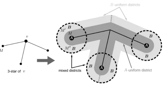
We establish that INDEPENDENT SET on planar cubic graphs reduces to WIN- NING DISTRICTS. We dene the mapping that assigns to an arbitrary planar cubic graphG= (V, E)a districting problem. We may assume that the graph is embedded in the plane such that all the edges are straight lines and denote the set of their midpoints by VE. We dene ε as the minimum of the distances between a point of V ∪V_E and a non-incident edge. The layout of the districts and the reduction can be seen in Figure 3.1. The 3-star of a vertex v ∈ V is the union of the three line segments betweenv and the midpoints of the three edges emitting from v.

Let the set of party A voters be V_E and with each party A voter M ∈ V_E we associate two partyB voters M⁰ and M⁰⁰ such that M⁰, M and M⁰⁰ lie in this order on the same straight line perpendicular to the edge ofM and the distance ofM⁰ and M⁰⁰ fromM is between ¹₅ε and ²₅ε.

For each midpoint M ∈ V_E we construct a party B winning district as the ²₅ε- neighborhood ofM. Since each of these districts contains two-party B voters and a partyA voter, so we call them mixed districts.

We associate with each vertex v ∈ V a party A winning district as the ¹₅ε- neighborhood of the 3-star of v. Observe that this district contains exactly three voters, and they are the midpoints of the edges ofv thus we call itA-uniform district.

Consider the set-theoretic dierence of the ²₅ε-neighborhood and ¹₅ε-neighborhood of the 3-star ofv, i.e., the subset of the plane consisting of the points having distance from the 3-star between ¹₅εand ²₅ε. This set contains exactly six voters, which are the partyB voters corresponding to the midpoints of the edges ofv. It is straightforward to see that the bisector of any angle dened by the edges atv and the edge dierent from the sides of that angle divide this set in such a way that each part contains

(48)

Figure 3.1: The layout of the districts. Source: Author.

three-partyB voters. We call these divided parts B-uniform districts.

Now, it is enough to show that the graph G has an independent set of size m if and only if the above-dened districting problem has a districting with m party A winning districts.

The sucient part of this claim is obvious since the partyAwinning districts of a districting are disjoint A-uniform districts, and they correspond to non-neighboring graph vertices.

For the necessary part, we construct for any given independent set of size m a districting havingm Awinning districts. Take theA-uniform andB-uniform districts corresponding to the vertices of the independent set and for the still uncovered voters, take their mixed districts. Clearly, all the voters are covered by a district, and it is not hard to see because of the choice of ε that the chosen districts are disjoint and each contains three voters.

We note that the associated districting problem described above can be determined in polynomial time.

(49)

The following easy consequence of Theorem 3.2.1 has practical importance.

Theorem 3.2.2. The decision problem whether a districting problem Π has a districting in which party A gains majority is NP-complete.

Proof. Note that all districtings in the proof of Theorem 3.2.1 have ³₂|V| districts.

Thus there exists a districting with at leastmwinning districts of partyA if and only if the following districting problem extended with dummy voters and districts has a solution in which the A winning districts form a majority. Let us add ³₂|V|−2m+ 1 extra disjointAwinning districts each containing three extraAvoters ifm≤ ³₂|V|/2, otherwise add 2m − ³₂|V|−1 extra disjoint B winning districts with three extra B voters in each.

Remark. The notion of majority in Theorem 3.2.2 is irrelevant. The same statement can be proved by analogy for any qualied majority.

3.2.1 A Positive Result

As we have seen in Theorem 3.2.1, nding an optimal districting is dicult. The problem becomes tractable if we replace R² with R in Denition 3.1.1, i.e., if we restrict the two-dimensional problem to a one-dimensional one. Observe that X and the admissible districts become intervals. For the sake of simplicity, we assume that X = [0, n], voter i is in the i^th unit interval, i.e., x_i ∈ (i−1, i), and the admissible districts have the form of[a, b]where a, b∈ {0,1,2, . . . , n}and a < b. If nis divisible by k, the problem of nding a partisan optimal districting is trivial. Therefore, in the remainder of this subsection we assume that n is not divisible by k. Then the admissible districts may contain eitherbn/kcordn/kevoters, which we will call short and long districts, respectively, and denote their lengths by s and l, respectively.

Based on the dynamic programming technique, we develop a polynomial time

(50)

algorithm that nds a so-called party A optimal districting for the one-dimensional districting problem.

For expositional reasons, we dene the indicator function w : D → {0,1} such that w([a, b]) = 1, if the district [a, b] is won by party A and w([a, b]) = 0, otherwise. We will keep a record of the variables W_i(j) (for j ∈ {0,1, . . . , n} and i ∈ {−1,0,1, . . . , nmodk}), which are initially all set to −1, terminating with the maximum number ofAwinning districts in a districting of the interval[0, j]in which there are exactlyi long districts if such a districting exists andi≥0.

Whenever W_i(j) ≥ 0 we dene p_i(j) as the starting point of the last district of one of the districtings corresponding toW_i(j).

The key observation is that from anA optimal districting of an interval[a, b]with a last district[c, b] we get anA optimal districting for the subinterval [a, c]by simply omitting last district[c, b]from the districting. Consequently,Wi(j)can be calculated fromW_i−1(j−l)and W_i(j−s), thus the following recursion hold:

W₀(0) = 0,

W₀(s) = w([0, s]),

while for(i, j)6= (0,0) and (i, j)6= (0, s) we have [W_i(j), p_i(j)] =











[Wi−1(j−l) +w([j−l, j]), j−l] if Wi−1(j −l)> W_i(j−s), [W_i(j −s) +w([j−s, j]), j−s] if Wi−1(j −l)< W_i(j−s),

[W_i(j −s) +w([j−s, j]), j−s] if Wi−1(j −l) = W_i(j−s)≥0 and w([j−s, j]) = 1,

[W_i−1(j−l) +w([j−l, j]), j−l] if W_i−1(j −l) = W_i(j−s)≥0 and w([j−s, j]) = 0,

[−1, −1] if Wi−1(j −l) = W_i(j−s) =−1, wheres < j ≤n and 0≤i≤n modk.

(51)

The values of w for short and long districts can be evaluated in linear time, while the calculation of the values W_i(j) is within O(n²) time complexity. Since k districts are required, the maximum number of districts party A can win is given by W_n_mod_k(n). The values p_i(j) can be used for reconstructing an optimal solution in linear time.

3.3 A Practical Approach

Since many NP-complete problems can be solved for real-life situations, we would like to point out in this section why it is dicult to nd an optimal partisan districting even if only a modest number of districts have to be formed.

A real-life knapsack problem can be solved in many cases, and the number of items together with the magnitude of their values describes the complexity of the problem well. Whereas the number of districts or the number of electoral wards for districting problems can be deceptive because, while the number of districts to be drawn is relatively small, the number of possible districts is already extremely large, as we will point out in the following paragraphs.

For instance, let us consider the Hungarian Electoral System in which since 2011, Budapest has to be subdivided into 18 electoral districts from a total of 1472 wards, each serving 600-1500 voters. Thus, an average district consists of approximately 82 wards. For simplicity, we model the election map by a 2-dimensional square grid, where every cell represents a ward with a given party preference A orB. Obviously, the real-life structure is even more complex because the distribution of partyAandB voters diers ward by ward, and there are further restrictions on the set of admissible districts. In this model, two cells are connected if they share a common edge, so this denes a 4-neighborhood relation on the set of cells.

Even in this simplied structure, there is no known formula for the number of

(52)

possible gures. It means, we do not know how many districts can be formed out of a given number of connected cells, so-called polyominoes. If even orientation matters, they are called xed polyominoes. It is known that the number of polyominoes grows exponentially. Jensen [34] enumerated xed n-cell polyominoes up ton = 56, which resulted in 6.9 × 10³¹ polyominoes for the last case, which equals the number of dierent shapes that can be formed out of 56 connected squares. This result shows that it is unfeasible to examine all possible cases, even for 82 wards on a Budapest scale problem. Therefore, in contrast to the knapsack problem, the number of districts to be formed in case of a districting problem underestimates the magnitude of the latter problem. Obviously, considering possible district shapes is just the rst step in arriving to a districting.

It is worth noting that the dynamic programming technique applied successfully for one-dimensional districting problems in Section 3.2.1, cannot be employed in exactly the same way for the two-dimensional problems specied above since, while for the one-dimensional setting, it was possible to evaluate any important subdistricting problem by simply omitting one small or one large district, from the explanations above it follows for the two-dimensional setting that the number of possible subdis- trictings will be simply too large, i.e., non-constant in the number of voters, to obtain a computationally feasible algorithm.

Another starting point to obtain a heuristic for gerrymandering, i.e., an algorithm which is not optimal but quick, would be the pack and crack principle. In a similar framework, Puppe and Tasnádi [56] showed that not every crack procedure reaches the optimal solution if geographical constraints are present. If the connectivity of the cells is not required, the problem can be easily solved by a simple crack algorithm, which leads to the optimal solution in this special case. The aim of the crack strategy for the beneciary party is to win the query district with just the least margin, thus