L A N D E V A L U A T IO N S TU D IES IN H U N G A R Y

(1)

(2)

L A N D E V A L U A T IO N S T U D IE S IN H U N G A R Y

(Studies in Geography in Hungary 23) Edited by

D. Lóczy

The Geographical Research Institute o f the Hungarian Academy o f Sciences has elaborated a method for determining cropspecific land suitability. The first part of this volume briefly describes this procedure and the way land suitability grid maps for individual crops are combined to show the areal distribution o f types o f agricultural habitat. The resulting regionalization is an important tool for regional planners since it portrays the allocation o f land resources on a simple map and promotes specialization.

The agroecological regions thus identified can. however, only reflect the physical potentials in the area. For a complex land evaluation this first stage o f the survey has to be supplemented with the assessment o f economic factors. As the complete methodology o f an economic evaluation o f land has not yet been elaborated for Hungary in a final form, an experimental method is presented here by L. Góczán (who has also guided the agroecological regionalization project). In the second part, he attempts to compute another numerical value incorporating gross crop production value, labour and capital investments as well as the numerical value o f the agricultural habitat.

(3)

LAND EVALUATION STUDIES IN HUNGARY

(4)

STUDIES IN GEOGRAPHY IN HUNGARY, 23

Geographical Research Institute Hungarian Academy o f Sciences

Editor in chief:

M. PÉCSI

Editorial board:

L. GÓCZÁN D. LÓCZY S. MAROSI 1. TÓZSA

(5)

LAND EVALUATION STUDIES

IN HUNGARY

Edited by DÉNES LÓCZY

AKA D É M IA I KIADÓ , BUDAPEST 1988

(6)

Revised by P. STEFANOVITS

Translated by E. DUDICH D. LÓCZY I. TÓZSA

Technical board:

K . EVERS, J. FÜLÖP, Mrs. ZS. KERESZTESI, M. M O LNÁR, J. NÉMETH, I. POOR, Mrs. E. T A R P A Y , Mrs. L. V ARG A

ISBN 963 05 5231 0 HU ISSN 0081-7961

( C ) Akadémiai Kiadó, Budapest 1988

Printed in the Geographical Research Institute Hungarian Academy o f Sciences

(7)

CONTENTS

PREFACE... y PART 1

GÓCZÁN, L. - LÓCZY, D. - MOLNÁR, K. - SZALAI, L. and' TÓZSA, I.: Agroecological Regionalization on the Basis of Suitability for Crop Cultivation: Example of Komárom County... 11 PART 2

GÓCZÁN, L . : A New Complex Procedure of Land Evaluation.. 77

(8)

(9)

P R E F A C E

Agriculture is an outstanding branch of the national economy of Hungary. The demand for agricultural produce is not limited to the nutrition of home population, but also observed in re

spect to the balance of foreign trade, considerably dependent on the exports of farming products processed at high levels.

Some crops and by-products are indispensable for industrial use and required in growing amounts.

The present economic reform in Hungary aims at introducing a new system of economic regulation, which is meant to en

courage the better utilization of environmental resources.

This increased reliance on natural potentials is indisputably imperative in field cultivation, where the control of environ

mental factors on production is the strongest and, supposing more appropriate economic regulation, the adjustment of pro

duction patterns to land capability would provide opportunities to raise profitability at relatively low levels of investment.

In order to plan the optimal use of land, up-to-date in

formation has to be available for the farms, on the quality of their land. The new land evaluation scheme under way rates tracts of land on a relative scale with numerical values of habitat ranging from 0 to 100 based on a nation-wide soil survey In the Geographical Research Institute of the Hungarian Academy of Sciences a method for determining crop-specific land suit

ability has been elaborated. The first essay of this volume briefly describes this procedure and the way land suitability grid maps for individual crops are combined to show the areai distribution of types of agricultural habitat. The resulting regionalization is an important tool for regional planners since it portrays the allocation of land resources on a simple map and promotes specialization, a desirable trend encouraged by the state.

The agroecological regions thus identified, however, only reflect the physical potentials in the area. For a complex land evaluation this first stage of the survey has to be sup

plemented with the assessment of economic factors. As the com

plete methodology of an economic evaluation of land has not yet been elaborated for Hungary in a final form, an experimental method is presented here by L. GÓCZÁN (who has also guided the agroecological regionalization project). In the second paper, he attempts to compute another numerical value in

corporating gross crop production value, labour and capital investments as well as the numerical value of the agricultural habitat. A modified variety of COBB-DOUGLAS' production function was selected to do this tasR and solved with the help of co

efficients of volume elasticity. Examples illustrate how the price of land is calculated for two farms of different ecologic

al endowments.

Both methodological studies are meant to contribute to the nation-wide survey of Hungary's most important natural wealth, fertile land.

Budapest, April 7, 1988

Dr Dénes Lóczy

(10)

(11)

P A R T 1

AGROECOLOGICAL REGIONALIZATION ON THE BASIS OF SUITABILITY FOR CROP

CULTIVATION: EXAMPLE OF

KOMÁROM COUNTY

László GŐCZÁN, Dénes LÓCZY, Katalin MOLNÁR, László SZÁLAI and István TÓZSA

Geographical Research Institute Hungarian Academy of Sciences BUDAPEST

(12)

(13)

1. INTRODUCTION

In Hungary the century-old, outdated 'Coldkrone' land evalua

tion, based on cadastral net income, is now being replaced by a new system.

The new evaluation system is launched by a government act and being introduced in two phases. In the first phase the qualities of the habitat limiting possible ecological yield are evaluated which are relatively constant components of the value of habitat.

The result of this agricultural habitat evaluation is the score value of habitat going to replace the old land value

index expressed in net income in the land registry.

The other, relatively fast changing, component of the score value of habitat is to be calculated through economic land evaluation. However, there is no established method for such evaluation yet.

Although promising experiments of elaborating complex land evaluation methods (BENET, I. - GÓCZÁN, L. 1973, a,b; NÉMET, L. 1970; SZŰCS, I. 1980a; FEKETE, F. 1984) taking into con

sideration the ecological differences in habitats (unlike the previous methods), have been made in the last two decades, they do not meet all the requirements of a modern land evalua

tion, since they do not include the land value component deriv

ed from the location-dependent land rent.

Calculating this location-dependent rent is rather diffi

cult in Hungary. On the one hand, state purchase prices do not include transport expenses, on the other hand there is no appropriate agroecological regionalization in the country which could render this calculation possible.

The lack of agroecological regionalization has a disadv

antage to the central planning of agriculture, viz. the elabo

ration of a rational land use model of the country required by a government decree.

2. CONCEPTS FOR DELIMITING AGRICULTURAL MICROREGIONS

Research workers undertook to set up an up-to-date agro

ecological microregionalization methodology, which is presented in tnis report and applied to one of the counties of Hungary.

István LÁNG, the secretary general of the Hungarian Academy of Sciences conducted a significant research project ("The agroecological potential of Hungarian agriculture by the turn of the millennium" 1979-82 - LÁNG, I. et. al. 1983) containing an agroecological regionalization of Hungary (GÓCZÁN, L.

NEMERKÉNYI, A., 1980), but it was actually the adjustment of the boundaries of the new physical geographical mesoregions (PÉCSI, M. - SOMOGYI, S. 1980) to the administrative divisi

ons. True agroecological boundaries were only dominant in the case of very prominent ecological contrasts. Naturally, physic

al geographical regions cannot be identified with agroecologic

al regions. The former represent more or less 'homogeneous' areas to the totality of physical geographical factors;

(14)

the latter are separable due to the degree of suitability for the ecological requirements of various plants.

Identifying agroecological regions cannot be restricted to only finding their boundaries, tracts of agricultural land has to be assessed from the viewpoint of its suitability for cultivation. The agroecological potential of a certain area can be revealed by deciding the most suitable plants to grow there and the degree of this suitability. In other words, the ecological suitability for crop cultivation of agricultural areas has to be decided. In doing so the chosen areal units should be applicable to agricultural co-operatives and state farms, e.g. 25 ha areal units are suitable as they answer the size of an average plot. As most information needed for the assessment can be derived from maps, the 25 ha areal units are to be constructed by overlaying a matrix (identified by x, y co-ordinates) on the maps.

In this way, however, the boundaries of agricultural farms are ,not observed, the total spatial agroecological data base of the country is going to be compatible to computer handling.

Such an agroecological regionalization method with proper, scientific viewpoints of suitability assessment remarkably reduces the subjectivity in defining^ the regions. During the suitability assessment the mosaics of the assessed 25 ha areal units are arranged into types of habitat in observation of spatial ecological regularities. Their homogeneous or hetero

geneous juxtaposition brings about objectively separable regi

ons.

The such constructed agroecological regions have more scien

tific and practical merit than regions constructed in any other way. Its first scientific and practical profit lies in its being an important tool to the new land evaluation.

The present cropland value score in the land register does not give any more information than expressing the relative quality of land compared with the best in the country. It does not give information about the crop to grow there and the suit

ability for its cultivation.

Our map of agroecological regions based on ecological suit

ability for crop growing, gives the above information for every 25 ha agricultural area.

In this sense, our agroecological regionalization method can promote and complement the land evaluation under way. An

other merit is its availability practically for every farm.

Its background data - for every 25 ha areal unit - are stored in computer files and can serve as a basis of a land informa

tion system too.

Finally, possessing suitability map the utilization and exploitation of ecological endowments can be monitored by digitally processed, satellite land use (crop pattern) maps.

Its importance for the central planning administration can hardly be overestimated.

3. LAND EVALUATION AND AGROECOLOGICAL POTENTIAL

The problem rises from judging the productivity of arable land. The expressions "land, habitat, soil, arable soil

(15)

productivity or fertility, capacity" are commonly used both in publicistic and professional literature.

The proper scientific expression in our case is the natural fertility of agricultural habitat and the productivity of agri

cultural habitat.

The natural fertility of agricultural land refers to the yield possible in a given area with constant physical (habitat) endowments, without applying any artificial nutrients and fertilizers and irrigation only relying on a simple agro

technique.

By constant habitat endowments we mean relatively stable properties of the following: soil type, soil subtype, textu

re, humus quality and quantity, thickness of humus layer, acid

ity, CaC O 3 content, leaching, organo-mineralic complexes and their adsorptional conditions, porosity, water capacity and permeability, eluviation and illuviation exchanging matter between soil horizons, thickness of fertile soil layer; parent rock, water supply, agroclimate and relief.

3.1. Agricultural habitats

In its original state, such an agricultural habitat is a natural ecotope. In our cultivated lands the agrotechnique, the organic residue of economic crops grown in rotation, not observing the boundaries of ecotopes and the enduring micro

climates of habitats, obscured the natural ecotope boundaries, and created agricultural habitats with similar - but no more identical - ecological endowments.

An excellent example for this in Hungary is the once homo

geneous ecotope covered by chernozem, formed on a westwardly exposed valley slope on loess parent rock. Half of it has kept its original thickness of humus layer due to contour observing mass cultivation, while the neighbouring small-plot slope cultivation area - which used to be the same ecotope - has become a completely eroded loess surface. Ramann's brown forest soil has been eroded down to the loess parent rock on the east- wardly exposed slope of the same valley. The present agri

cultural habitats include the divergences of once identical ecotopes and the convergences of once different ecotopes.

3.2. Agroecological potential of an agricultural habitat

It means the actual fertility of cultivated land having been affected by some agrotechnique. This potential depends on the way the habitat responds to ecotechnical, agrotechnical and agrochemical effects and the degree of possible economic effectiveness of these effects on a given, modern technical level of production. This productivity can be called agro

ecological potential.

Every country and national economy is basically interested in preserving the agroecological potential of the cultivat

ed land.

Central planning authorities are also interested in sub

dividing agricultural land with similar agroecological potent

(16)

ials, so as to be able to incite economy to obtain more profit and land rent obsessing the best ecological endowments through specialization.

Agroeconomics is concerned with differences in land quality when stating the differential rent or the differential net in

come. Actually it means the geographical differences in the agroecological potential of cultivated land.

To measure these differences, first the quality criteria of the best habitat properties in the country have to be established so that the score value of habitat can be compared with it.

The simplest and most reliable way of accomplishing it is to compare the endowments of the cultivated land with the average crop yields. The average of the inter-war period should be selected for reference, as chemical fertilizers did not affect the quality of arable land then.

This comparison offers a rating possibility which assigns maximum ranks to the best habitats (with the highest crop yields at a given agrotechnical level) and minimum ranks to the worst, infertile lands.

All the different quality habitats can be rated proportion

al to their value between the best and worst (highest and lowest scores on the score range) cultivated lands.

3.3. Land evaluation concepts

This concept has been realized in several countries (TEACI, D. - BURT, M., 1974) and in Hungary too, with an agricultural land evaluation using scores from 0 to 100. Its implementa

tion was made compulsory by a resolution related to the Land Act as- mentioned above (In: Mezőgazdasági és Élelmezésügyi Értesitö, August 22, 1982).

This land evaluation is bas^d on the preconception that the genetic and other productivity-affecting properties of soils represent about 90% of the other physical factors control

ling the fertility of the habitat. It is expressed in the score range assigned to the soil subtypes. During the further evaluation only those partial ecological effects are taken into consideration which are not represented by soil properties.

For instance, the quantitatively evaluable surface water loss .due to relief is not reflected in the genetic character

istics of soil, so this effect is represented by a correct

ional score amounting to only 5 % of the maximum value score of habitat.

The evaluation of the ecological potential in an agri

cultural area can be approached without emphasizing a dominant factor (like soil) in the productivity of the agricultural habitat. Under different physical geographical conditions on certain cultivated lands different ecological factors may prove to be favourably dominant or restrictive from the viewpoint of crop yield.

That is the reason why - according to this concept - the different types of agroecological factors are provided indi

vidually with the customary scores ranging from 1 to 100.

(17)

This kind of agricultural environmental assessment results in the areal survey of six main agroecological factors. The factors are referred into 10 categories and supplied with rank scores in a square-grid system representing areal units.

This assessment gives more information than the value score of habitat inasmuch as it provides us with information about the quality of agroecological factors separately. It defines the planning for the necessary interference to ameliorate culti

vated land (GÓCZÁN, L. et a l . 1979).

Both methods may have two disadvantages from the viewpoint of agricultural users:

- None of them expresses the absolute (economic) value of the arable land, or the way to calculate it.

- None of them gives information concerning the crop-speci

fic relative suitability of land, or the degree of this' suitabi1ity.

3.4. A complex land evaluation

Experiments have been made to remedy of the first inadequacy.

The score value of habitat e.g. (STEFANOVITS, P. et al. 1974) is to represent the contribution of land (one of the factors of cultivation) to agricultural production value. The economic value of land could be calculated if the value score of habitat defined the developing ratio of net income in long-term average, or the total value of agricultural production of labour and capital in an unit area. Such an experiment was first conducted by Iván BENET and László GÓCZÁN. As internationally the first complex land evaluation method, it made a real land value calcu

lation possible in an economic system where - due to collective land ownership - there is no regulated land market yet. This method defines the yield quota (of the cultivated land) from the threefold production result of land-capital-labour with a Cobb-Douglas type production function adapted to 3 independent variables; it considers the gross plant production value as the result variable and the computing the elasticity coeffici

ent for the land represents the land productivity in percentage.

The formula is:

y = a F ^ K f where

y is the gross plant growing value of a cropland;

F is the cropland score propositioned by the size of the land;

L is the cost of live labour in forints;

K is the cost of capital for each field in forints separate

ly the basic capital (K^) and the basic capital (K^);

a is proportion factor

c*,/3,X = elasticity coefficients representing the yield-quota of land, labour and capital;

cx+ß-t f = 1 expressing the volume elasticity of production.

The land elasticity coefficient of the correlation matrix solved by the above formula for all the fields of an agri

cultural farm will give the price of the areal units of the farm if the land elasticity coefficient is weighted by the crop growing value and its capitalized sum by the rate of in-

(18)

terest of long-term deposits. Authors chose this land evaluat

ing method because in the socialist economy the transportation expenses - due to uniform prices - do not influence the prize of crops; so there was no need for computing the components of either positional or differential ground rent.

3.5. Modifications

The Economic Land Evaluating Council of the Hungarian Acade

my of Sciences, formed in 1981 for the implementation of the government decree considering the establishment of a new eco

nomic land evaluation method, decided to have the economic value of agricultural fields determined by the net income of crop returns and by calculating the differential rent.

The Methodological Committee, formed to introduce the method, accepted Iván Benet's and László Góczán's land evaluation method among several others with a few important changes.

These alterations include, for instance,

- that the net income was accepted in the function as a result variable (instead of the gross plant production value)

- the Benet-Góczán function of 3 independent variables was developed into a function of 5 ones (to indicate the effects of amelioration and irrigation)

- economic data sequences were considered in the correlation matrix instead of data sequences for fields recorded by the farms.

This study is not meant to present the above method in more detail, nevertheless, the first author summarizes his comments to it:

- The account of net income for farms is rendered quite unreliable by the different promotional forms and counter- interests of farms.

- The data acquisition of the 5th independent variable introduced to display the effects of amelioration and irriga

tion is quite uncertain, and it is only of additional import

ance composed with the 3 main production factors. The sub

ordination scale of the 4th and 5th variables differs from that of the first 3 ones among one another. Therefore, the interpretation is made unreliable.

The land elasticity coefficient of the correlational matrix of economic data sequence permits the defining of the average value of farm land and not the real value deriving from the quality differences between fields. So the economic land evaluation does not serve its purpose and even shows the false image as if a modern economic land evaluation was established.

- Nor can the differential land rent be defined by this method, as only a reliable ecological regionalization makes the computation of positional land rent possible.

- Our study aims at eliminating the second obstacle by the introduced two agricultural environmental assessment methods.

(19)

4. AN AUTOMATED ASSESSMENT OF LAND SU ITABILITY

4.1. Land evaluation approaches

In international literature (McRAE,S.G. - BURNHAM,C.P. 1981) the following approaches to agricultural assessment of the physical environment (Land evaluation) are known. The assess

ment may be direct, based on crop yields, although in this case we have to consider numerous social and economic factors, too. The indirect approach tries to characterize crop-specific land sutability or land capability for different crops and their relative order through some system of comparison. The actual classification is either based on the threshold value of some important factor (as in the case of category-systems), or on evaluating numerous parameters (parametric systems).

The system introduced in this study is parametric (considers the conditions of factors). There are both disadvantages and advantages of such a method. Although parametric systems are quantitative, accurate and specific, easy to apply and simply constructed (in our case for certain crops) but they require multifarious knowledge in the earth sciences (pedological, agroclimatoiogicai, geological ets.) so their objectivity and accuracy depends on the exactitude of this knowledge.

The parameters can easily be transformed, changed, increasing perhaps their subjectivity thus to achieve an expected "good"

result. One might express a subjective opinion in the language of mathematics. The restrictions should also be considered along with the requirements. One of the main characteristics of such systems is computing a great variety of factors collect

ed into computer data bank. The interactions between factors are imperfectly understood (quantitatively) so their integration is not reliably established either. Land evaluation may serve taxation and regional planning and natural resources surveys very well but, once it is codified legally, it can hardly be changed. It can be applied to the field units of farms although its areal validity is not extensive and it can only be mapped in the form of combined categories. In the parametric systems the score values of factors can either be integrated through addition or multiplication or both. The additive method was applied to the investigation of Komárom county although there were multiplicative experiments too which require more reliable data but can show more detailed areal differences (GÓCZÁN, L. - HARNOS, Zs. 1980, SZALAI, L. 1987).

The method to be introduced in the following springs from a three-author study (LÓCZY, D. - TÉCSY, Z. - TÓZSA, I. 1981) written in the Geographical Research Institute Hungarian Academy of Sciences for a competition call. The method of the study has been developed by the authors in several steps (LÓCZY, D. 1982), using a previous soil survey as a primary data base

(GÓCZÁN, L. et al. 1969), into a level which might be suitable to achieve the above-stated goal.

It is a new environmental assessment method which classifies the present condition of physical environment (affected by usual agrotechniques) by areal units (in this case 25 hectares) into ten intervals from 0 to 9, from the viewpoint of a given land use (or ecological land capability). The method can be

(20)

listed among the suitability surveys or site analyses, as cited in English literature (HOWELL, E.A. 1981).

4.2. A brief survey of the method

Once the purpose of assessment is defined, the steps of the suitability analysis are the following (LÓCZY, D. 1982, 1984):

- establishing a computerized data base

- defining and collecting the suitability indices - elaborating the assessment algorithm and programme

- automated display and printing of the assessment map.

First data have to be acquired concerning the conditions of all agroecological factors which affect crop growing. These data are required to establish the suitability degree of the factors regarding the ecological demands of crops.

Similarly, the ecological demands of the crops to assessed are also to be collected with special concern to the demands

in critical periods of their growing seasons.

The third and the fourth steps are executed by a programme writer assistant and a computer.

4.2.1. Computerized data base of assessment

Only a computerized data base can promote an environmental assessment with agricultural viewpoint and enable it to display the ecological suitability for cultivation in an agricultural area in a cadastral survey.

4.2.1.1. T h e s q u a r e - g r i d s y s t e m f o r a c q u i r i n g a n d s t o r i n g d a t a Many factors have to be considered in a studied area to characterize the physical environment. With the help of a dense grid system sufficient data have to be collected on field. These data can be presented on chorograms (adjusted into categories). The information of separate chorograms can

not simply be unified by their superposition, as spatial dis

tribution patterns vary with different factors. The areal validity (extension) of field data is limited according to the professional experience of the investigator. The inaccuracy emerging from this fact cannot be neglected even with the most experienced mapmakers. Therefore, when superposing choro

grams, the border lines of units may separate such areal units which, in reality, are hardly different from the neighbouring ones. The lucidity of integrated maps is rather bad due to their fragmented appearance. This potential error is increased if the superposed chorograms are constructed from maps of various scales through enlargement or reduction (as it often happens though in data acquisition).

The solution can be a simple, constant reference basis independent from the spatial distribution of physical factors, which can "unify" numerous chorograms. A standard square- grid system (KLINGHAMMER, I. - PAPP-VÁRY, A. 1973) can be imposed on every chorogram and the coincident square units of all factors can be referred to the same way. The squa re

(21)

grid data acquisition, storage and retrieval system meets the above requirements. As every method, with its advantages, it has its disadvantages too. The border lines of different qualities are approximative. Consequently, they are rather inaccurate on the square-grid map. However, the lines of the grid function as border lines concerning parameter values and the spatial distribution of several factors and the posi

tion of a square can easily be recognized. By placing the grid system upon the chorograms, they can be digitized without difficulty extending the dominant figure (quality) throughout the whole square unit. A figure is written into each unit of the square-grid. The data matrix of an adquately detailed square-grid can reflect the spatial distribution of factors reliably. The scale depends on the survey goal and the density of the data available. The areal units can be identified by indicating the rows and columns with figures or letters. The origin of such coordinate system is arbitrary but in the case of a national survey it can be made uniform. One of the dis

advantages of the square-grid system is its inaccuracy compared to ordinary maps, and that exact areal extensions cannot be calculated from them. The approximate size of areas can easily be seen and defined by summing up the square units.

Used as overlays, the grid maps even increase the minor inaccuracies of the chorograms and the 'border effect', known from the interpretation of satellite images, can be observed (i.e. false results appear along the margins of homogeneous areas).

4.2.1.2. A c o m p u t e r c o m p a t i b l e d a t a b a s e

When all the required, digitized maps are brought together in a square-grid map sequence, the uniform data file can be stored in computer memory.

Not all the chorograms used in environmental assessment, however, are based on numerical information. The chorograms of the parent rock or land use do not show figures but various qualities (like loess, sand or meadow, settlement, etc.).

The categorized numerical data and the qualities identified with names can only be stored in a uniform way with the help of coding. The possible conditions of the chosen physical factors in Hungary are represented by code numbers in some logical order. The II.10/10 symbol means the 10th factor (e.g.

the temperature total for October expressed in °C) and its 10th condition (331-340°C); and similarly the III.20/10 symbol means the 20th factor (e.g. physical soil type) and its 10th condition (sand soil), which are not numerical conditions.

A code often represents the combined conditions of factors.

In such cases a coding table is needed to encode the condi

tions or qualities. Actually, the data base should not only record the conditions of isolated factors, but at least the most important interrelationships too. The factors closely related to each other can be stored together in the memory also saving computer running time thereby.

The method has to meet the requirements of data storage and retrieval, because the multifactoral assessment of the

(22)

physical environment needs such large amount of data that can only be handled by computer. After having the assessment programme run, the plotter of the computer can print the as

sessment 'map' derived from data base, in the form of a data matrix similar to the form of the stored data files. The syn

chronous printing of the code numbers of a factor or two is possible if we want to compare them. Mathematical statistical relationships can also be computed between them.

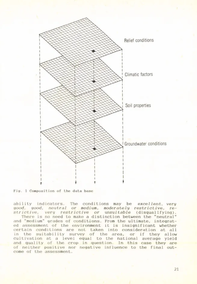
Figure 1 shows the data base set up of superimposed square- grid maps.

The code numbers of the factors required for the assessment are present in the data base. Apart from the extent of the area to be assessed, two conditions define the size of the data base: all important factors should be present (codes have to be assigned to all of their states occurring in Hungary even if they are not to be found in the investigated area), and the properly detailed data of the factors should be acces

sible either on thematic maps or through simple field in

vestigation.

A data base compiled for a given assessment goal can be used partially or as a whole for an assessment with a different goal. (Supposing the data are sufficiently detailed from the viewpoint of the new goal./ To ensure this, no assessment score should be assigned to the stored codes. The data base (i.e. the area portrayed by the coded parameters) has to be assessed by a computer programme. This programme is to be changed as necessary with the changing goal. The data base is supplemented with the codes of the new factors. The judge

ment of the old elements often changes in the new programme.

If, for instance, the 6/11 (the 11th condition of the 6th factor) was "good" in one assessment. It may, in turn, be "re

strictive" in another.

The data base is increased with the addition of new assess

ment goals, reflecting the physical environment more and more comprehensively (although never in an exhaustive manner).

The superimposed square-grids illustrate the digital storage of the conditions of environmental factors.

4.2.2. Identifying suitability indicators

Whatever the purpose of the environmental assessment should be, its efficiency is basically influenced by the rate of accurate and unambiguous definition of the requirements set up by the economic branch utilizing the physical environment.

One of the viewpoints in constructing the data base is the factor to which the utilizing economic branch or other activity is the most sensitive. The user itself should 'hand in' the list of the favourable and unfavourable conditions which limit the suitability of the surveyed area from the viewpoint of the assessment goal.

The data base is the 'supply' side of environmental assess

ment, while the requirements of the user constitute the 'demand'. The link between them is the sequence of the suit

ability indicators. Their task is to confront the demands and the endowments of the area on the level of well-defined, elementary environmental conditions. The conditions of the environmental factors are actually categorized by the suit-

(23)

Relief conditions

Climatic factors

Soil properties

Groundwater conditions

Fig. 1 Composition of the data base

ability indicators. The conditions may be excellent, very good, good, neutral or medium, moderately restrictive, re

strictive, very restrictive or unsuitable (disqualifying).

There is no need to make a distinction between the "neutral"

and "medium" grades of conditions. From the ultimate, integrat

ed assessment of the environment it is insignificant whether certain conditions are not taken into consideration at all in the suitability survey of the area, or if they allow cultivation at a level equal to the national average yield and quality of the crop in question. In this case they are of neither positive nor negative influence to the final out

come of the assessment.

(24)

Regarding their contents, the suitability indicators are correlations between (quasi)elementary environmental con

ditions and suitability grades. They can be listed in tables from which we can learn how the coded conditions meet the demands set up by environmental management. E.g.:

factor excel- very good medium no lent good

moderate- restrict- very unsuit- ly re— ive restrict— able

strict- ive

ive

19 3 4 2 6 5 1 7

Here the 6th condition of the 19th factor is judged to be neutral or of medium quality and, thus, it does not influence the evaluation.

The 'unsuitable' label does not automatically mean complete overall unsuitability. The assessment programme has to be designed to assess an unit where an unsuitable condition oc

curs, worse than neutral.

The grades of suitability can naturally be increased depend

ing on the completeness of the list reflecting the users' requirements. The above table with eight classes (including the 'neutral' classification) seemed to be sufficient for an experimental run of the method.

We do not have to find suitability indicators for every environmental condition, and, similarly, we do not have to consider every factor for each assessment goal.

After making up the list of suitability indicators we have to mark those factors which are to be emphasized in the auto

mated assessment, according to their prominence in the total environment. These are the climatic parameters for critical months or the most compound, complex of factors, the genetic type of soil. The rate of weighting (twofold or fourfold) in the assessment programme, has to be decided from experience.

4.2.3. Assessment algorithm and programme

Having enlisted all the important conditions of all the important factors into suitability rates by the classification of code numbers, and having both the data and the suitability indicators in the input data, we have given the computer all the necessary information to complete the assessment. From now on the environmental assessment can be fully automated.

The assessment algorithm contains the steps of mathematic

al data processing. It means the order of comparing all the units of the data base codes to the suitability indicators.

A programme is written on the basis of the algorithm in some computer language (in our case in BASIC). It orders the corn-

(25)

puter to assess each unit. According to the suitability cate

gory to which each localized condition (code number) belongs, the programme marks the units with scores from +3 to -12.Having repeated the procedure for each factor it considers their weighting and adds up the figures. The resulting series of figures from the small to the greater numbers are subsequently categorized from 0 to 9. These scores are assigned to the areal units, they are the rank scores representing the final score of the units.

0 means that the areal unit is unsuitable for the given specified utilization and 9 represents the best under the conditions of Hungary. The other scores are proportional to the dgrees of relative suitability.

4.2.4. Ecological suitability plotted by computer

Having assigned a rank score (from 0 to 9) to each areal unit, the computer plots the environmental assessment matrix with the help of the coordinates of the areal units. The inter

vals of printed figures can be fixed so that the figures should match into a square-grid of the desired size. This way we can obtain a digitized 'grid m a p ’ of similar scale to that of the data matrix. However, the vertical scaLe cannot perfect

ly be adjusted to the horizontal one.

We can render our 'map' more expressive by colouring the squares according to the figures (e.g. from the cold colours towards the warmer) and we can demonstrate increasing suit

ability through this. Figures make the mathematical inter

pretation easier, while displaying in colour promotes the visual one.

5. THE SCALE OF ASSESSMENT AND LIMIT OF AREAL ERROR

Any land evaluation with agroecological purpose has to observe the interests and conditions of agriculture. In crop cultivation the smallest unit is the field so, in theory, data collection and evaluation have to have areal units smaller than the smallest field. Farming units may also be interested in the differences within the area of a single field actually.

The smaller the units are, the more precisely the fields can be displayed in the 'square-grid maps'. In the case of land suitability for the area of one farm, surveying a few dozen hectare fields, the squares cannot be larger than 10 ha. Since this detail, if applied to several thousand sq. km areas, would not be maintained on a personal computer, a reduced scale had to be found.

In our expriment the scale was 1:25,000 which means 25 ha squares, using sq. cm units in the printed square-grid system.

The data sources available for the present study enable us to use this scale.

When digitizing the maps, we have to be aware of the fol

lowing sources of error:

a. The size and shape of an area spot changes on the square- grid map. The error depends on the positioning of the square-grid. However, the difference is not very signif-

(26)

icant, it is about 5% with an area larger than 100 hectares.

The increases and decreases for individual fields level each other out in the end product.

b. Areal units, smaller than half of the square-grid (ca 15 hectare) can be neglected. The square-grid 'map' is naturally more generalized than an ordinary chorogram.

c. "Averaging" the conditions of environmental factors (which is necessary to digitize map content square by square) is more difficult when we consider iand qualities as gen

etic type of soils, or parent rock than we consider 'quan

titative states' (as slope category and soil pH). When a square is located on the boundary of two different areas of a map it is difficult to decide the code to be assigned to the square. The error can be decreased if this situation is repeated so that we can take turns in digitizing the conditions. This way the proportion does not change over larger areas (Fig. 2).

d. The also manifest 'border effect' has already been de

scribed.

Fig 2 Coding environmental conditions (example: parent rock) differing in quality.

1 * code for sand; 6 = code for clay. Areal error is + 4.2 per cent

Somewhat simplifying the previously applied system (LÓCZY, D. 1984), we selected 21 environmental factors (Table 1) for the land suitability survey. We studied the very detailed spati

al distribution of 6 of them. The areal error limit of the whole data base is estimated at not more than 10 per cent.

(27)

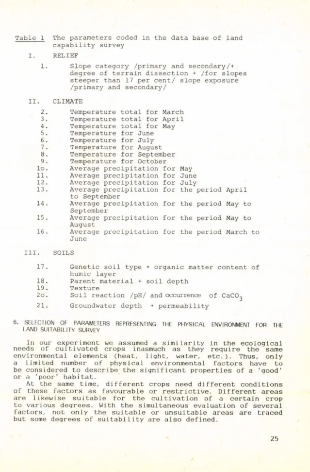
Table 1 The parameters coded in the data base of land capability survey

I. RELIEF

1. Slope category /primary and secondary/+

degree of terrain dissection + /for slopes steeper than 17 per cent/ slope exposure /primary and secondary/

II. CLIMATE

2. Temperature total for March 3. Temperature total for April 4. Temperature total for May 5. Temperature for June 6. Temperature for July 7. Temperature for August 8. Temperature for September 9. Temperature for October

10. Average precipitation for May 11. Average precipitation for June 12. Average precipitation for July

13. Average precipitation for the period April to September

14. Average precipitation for the period May to September

15. Average precipitation for the period May to August

16. Average precipitation for the period March to June

III. SOILS

17. Genetic soil type humic layer

+ organic matter content 18. Parent material + soil depth

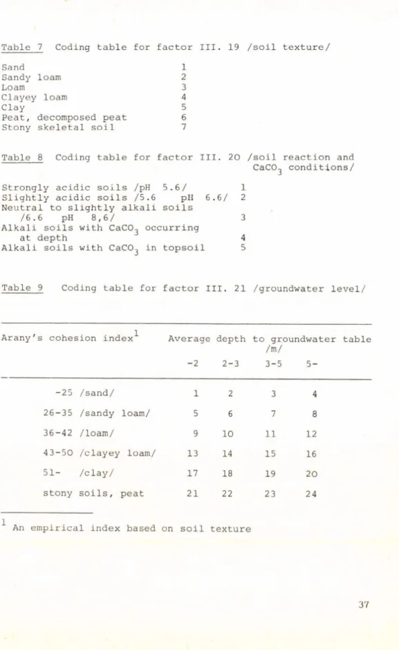
19 . Texture

2o . Soil reaction /pH/ and occurrence of CaCO^

21. Groundwater depth + permeability

6. SELECTION OF PARAMETERS REPRESENTING THE PHYSICAL ENVIRONMENT FOR THE LAND SUITABILITY SURVEY

In our experiment we assumed a similarity in the ecological needs of cultivated crops inasmuch as they require the same environmental elements (heat, light, water, etc.). Thus, only a limited number of physical environmental factors have to be considered to describe the significant properties of a 'good' or a 'poor' habitat.

At the same time, different crops need different conditions of these factors as favourable or restrictive. Different areas are likewise suitable for the cultivation of a certain crop to various degrees. With the simultaneous evaluation of several factors, not only the suitable or unsuitable areas are traced but some degrees of suitability are also defined.

(28)

Describing land suitability was first set as a goal in a soil survey (KREYBIG, L. 1937, pp. 6-7.): "The volume (financial value) of the investment required by the largest possible yield and by the needs of different crops defines the production

value of soils." #

"If we want to decide which agricultural production system and method can be applied the most successfully ... we have to know the ecological needs of plants, the most important soil properties, the climate and the weather and all the laws of nature prevailing in the relationships between soil and plant life."

This quotation emphasizes the relationship between the eco

logical value of the agricultural habitat and the applied agro

technique and profitability.

G. GÉCZY conducted a national soil use mapping in 1957-1968.

Its purpose was to find the crops with the highest suitability for certain soil types. The endowments of agricultural habitats were referred to five grades according soil use groups (GÉCZY, G. 1965).

The present system, which heavily relies on previous research (including the land evaluation project), identifies 8 classes

"excellent, very good, good, medium, moderately restrictive, restrictive, very restrictive, unsuitable" and refers environ

mental conditions to them according the degree to which they meet the ecological demands of crops. In practice, it means the increase or decrease of national average yields at a uniform level of agrotechnology, caused by the environmental conditions in question.

If data from experiments were available on the relative significance of individual physical factors in crop develop

ment about their influence on crop yields and quality, the present relative rating could be made more sophisticated through increasing the number of classes. Theoretically, it is feasible to determine ecological requirements in experiments (see, for instance, TEAC1, B. - BURT, M. 1964). The impact of each factor judged important would be measured against the average con

ditions of other factors. (The principles and stages of agro- meteorological and phenological observations are described by VARGA-HASZONITS, Z. 1977.) The interactions between factors could also be revealed in more detail. If the results of experi

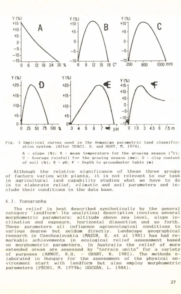
mentation, i.e. the crop yields were plotted against various parameters investigated on a chart, a more objective foundation could be given to the suitability indicators (Fig. 3).

However, until such detailed empirical findings are availab

le, the information gathered from literature (which is occasion

ally ambiguous or even contradictory) have to be relied on, (see Bibliography).

The main groups of ecological requirements according to sources in literature are

a) certain relief parameters;

b) agroclimatological elements;

c) soil properties. *

*

Simply meaning the way of cultivation. The term was not conceived in its modern sense at that time. (L.D.)

26

(29)

Fig. 3 Empirical curves used in the Romanian parametric land classific

ation system. (After T E A C I , D. and BURT, M. 1974).

A = slope (S>); B = mean temperature for the growing season (*C);

C = Average rainfall for the growing season (mm); D <* clay content of soil ( 3 s ) ; E = pH; F - Depth to groundwater table (m)

Although the relative significance of these three groups of factors varies with plants, it is not relevant to our task in agricultural land capability studies what we have to do is to elaborate relief, climatic and soil parameters and in

clude their conditions in the data base.

6.1. Topography

The relief is best described synthetically by the general category ’landform'. Its analytical description involves several morphometric parameters: altitude above sea level, slope in

clination and exposure, horizontal dissection and so forth.

These parameters all influence agroecological conditions to various degree but seldom directly. Landscape geographical research in Czechoslovakia (MAZÚR, E. et al 1981) has had re

markable achievements in ecological relief assessment based on morphometric parameters. In Australia the relief of more extended areas are assessed by "terrain units" for a variety of purposes (ARNOT, R.H. - GRANT, K. 1981). The methods e- laborated in Hungary for the assessment of the physical en

vironment start with landform but also employ morphometric parameters (PÉCSI, M. 1979b; GÓCZÁN, L. 1984).

(30)

In the method for determining land suitability for crop cultivation a less complicated approach should be adopted.

Not more than a single relief factor can be included unless relief were overemphasized in the end product of the assess

ment. Additional factors would be unnecessary overburden for the data base and would finally make computer processing un

economical .

Landform elements have significance, first of all, in three respects: they influence microclimate, control soil depth and the position of groundwater table. The last two are considered with the soil properties, but the microclimatic influence,

in lack of microdynamic data, has to be taken into account when assessing relief. Landforms build up of slopes and flat surfaces; describing them by parameters is equivalent to giving them names. Consequently, the relief factor employed in the system is based on slope inclination and, in the case of slope angles above 17 per cent, complemented with slope exposure.

Since the areal units of the microregional subdivision survey were larger than previously (25 ha squares), secondary slope inclinations and exposures were also taken into account. The percentage slope categories equal to the classes generally applied in agriculture (ERÖDI, B. - HORVÁTH, V. 1965). The requirements of agrotechnology, mechanization are reflected in the classes. Eight points of the compass were differentiat

ed in a grouping accordant with microclimatic influence (S and SW; W,E, SW and SE; N and NE).

The coding of relief conditions is presented in Table 2.

In the assessment of relief vertical dissection (relative relief), although important mainly in agrotechnology, was neglected. Field cultivation in Hungary is limited to a rather narrow altitudinal zone (ca 80-350 m above sea level). Within that, slope category is the most important cause of variation.

As a matter of course, topography reappears in the assess

ment with soil properties, the map representations of which are adjusted to relief (particularly in the case of the depth of humus layer - parameter no 18 in Table 1).

Minor relief is able to exert a decisive influence on soil formation and erosion. The independence of the relief factor is, therefore, relative, as it is bound to other factors at the various stages of the assessment procedure.

6. 2. Climate

In our method climate is assessed at macro and mesolevels.

It would be too expensive to carry out microclimatic measure

ments of proper detail (photosynthetically active radiation, soil temperatures at various depths, etc.), but further im

provement of the evaluation would inevitably call for the data of representative test areas (JAKUCS, P. - MAROSI, S.

- SZILÁRD, J. 1969) and their extension through analogy.

At present, the most direct climatic modification by relief should appear clearly (see above at the relief factor).Applying the long-term observation theories of meteorological basic stations through interpolation with regard to physico-geographical principles, reliable data can still be gathered

(31)

Table 2 Coding table for factor I. 1/Relief/

Subordinate slope category %

>25 17 - 25 12- 5- 0- none -17 -12 -5 Subordinate slope exposure

S W N S W N

E E

Predam- Dissection inant

slope expos

ure m/25 ha

Predom

inant slope categ

ory

%

SW SE NE SW SE NE

NW NW

(32)

for areas of some dozens of 'sq. km (for arbitrarily delimited areas as the administrative areas of villages).

Originally, we attempted to break down the agroecological significance of climate to its three major components, the dominant climatic factors: radiation, temperature and water budget, since the degree to which the energy and water demands of plants are mapped is a primary indicator of land capability

(VARGA-HASZONITS, Z. 1977).

The method for identifying climatic regions by the value of energetical potential production (the amount of carbohydr

ates produced at 5 per cent efficiency level of photosyntheticab ly active radiation - elaborated by SZÁSZ, G. 1979) was aband

oned and not included among the factors controlling land suit

ability, since it itself involves regionalization.

In the agroecological literature the temperature and water requirements during the growing season of cultivated crops are indicated. The indicators for the whole growing season are not informative enough to be used in land suitability investigations, since if a crop requires 2600 to 2900 °C temperature during its growing season, it does not mean more than the mentioned crop can be cultivated safely in Hungary.

However, in the development of each plant species there are one or more periods when the plant is particularly responsive to the factor of the external environment, including climate.

The temperature requirements of crops are only considered during these periods termed critical in agrometeorology. In agroecology the critical periods (phenophases) are approximat

ed by two-week on ten-day spells (decades). In land suitability studies this detail cannot be attained, since data can only be gathered for months (and long-term averages are also cal

culated for months). Consequently, the temperature of the critical months of the growing season (from March to October) are analysed and included in memory (Table 3).

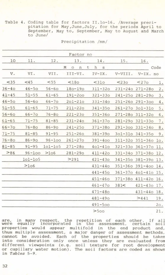
There are critical months o%f the water supply of plants too and monthly rainfall figures also appear in the data base coded according to Table 4.

To allow for total precipitation during the growing seasons of root crops, various perennial crops and winter cereals, additional parameters were included.

Available moisture from precipitation depends on runoff, infiltration and water capacity conditions. Runoff is regarded approximately proportional to slope category and, therefore, was not considered again. Infiltration is a function of soil permeability. Soil texture classes are regarded to ensure reliable coding.

Some agroclimatic indicators of lesser importance (wind direction« and velocity, cloudiness, vapour pressure, winter temperature and precipitation) were not included into the assessment at all. The remark should be made here that in the land suitability analyses for the cultivation of certain crops (for instance grapevine or fruit-trees) the incorporation of other climatic elements (as frost hazard) cannot be avoided.

The extremities of weather are even more effective on plant development than climate. Although the assessment of weather is outside the scope of the present system, a future perspect-

(33)

Table 3 Coding table for factors II. 2-9./Temperature totals for the months of the growing season/

Temperature totals /°C/

Factor no

2 3 4 5 6 7 8 9

M o n t h s Code

III. IV. V. VI. VII. VIII. IX. X. no

<loo <2oo <35o <45o <55o <5oo <4oo <25o 1.

lol-llo 2ol-21o 351-36o 451-46o 551-56o 5ol-51o 4ol-41o 251-26o 2 111-120 211-22o 361-37o 461-47o 561-57o 511-520 411-420 261-27o 3.

121-13o 221-23o 371-38o 471-48o 571-58o 521-53o 421-430 271-28o 4.

131-140 231-24o 381-39o 481-490 581-590 531-54o 431-440 281-29o 5.

141-15o 241-25o 391-4oo 491-5oo 591-600 541-55o 441-45o 291-3oo 6.

151-160 251-26o 4ol-41o 5ol-51o 60I-6I0 551-560 451-46o 3ol-31o 7.

161-17o 261-27o 411-420 511-520 611-620 561-57o 461-47o 311-32o 8.

171-18o 271-28o 421-43o 521-53o 621-630 571-58o 471-48o 321-33o 9.

181< 281-29o 431-44o 531-54o 631-64o 581-59o 481-490 331-34o lo.

291-3oo 441-45o 541-55o 641-65o 591-600 491-5oo 341-35o 11.

3ol-31o 451-46o 551-560 651-66o 60I-6I0 5ol-51o 351< 12.

311-320 461-47o 561-57o 661-67o 611-620 511< 13.

321-330 471-48o 571-58o 671-68o 621-63o 14.

3 3 K 481-490 581-59o 681< 631-64o 15.

491-5oo 591-600 611-65o 16.

5ol< 6ol< 651-660 17.

661< 18.

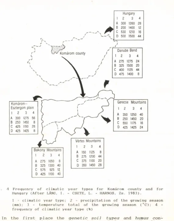
ive exists starting from the frequency of year types of dif

ferent weather conditions (atlantic, continental or mediter

ranean). A comparison of the national and regional (for the test area of Komárom county) frequency values is shown in Figure 4.

6. 3. Soils

While mesoclimate is uniform over large surfaces, soil endow

ments are distributed in a mosaical fashion. Soils are the most diverse components of the physical environment.

Soil surveys apply numerous parameters to portray the soil conditions of an individual area. The maps produced

(34)

Table 4. Coding table for factors H.lo-16. /Average preci

pitation for M a y ,June,July, for the periods April to September, May to, September, May to August and March to June/

Precipitation /mm/

Factor no

10 11. 12 . 13 . 14 . 15 . 16 .

M o n t h s Code

V. V I . VII. III-VI. IV-IX. V-VIII. V-IX. no

<35 <4 5 <55 <18o <31o <23o <27o 1.

36-4o 46-5o 56-6o 18o-19o 311-320 231-24o 271-28o 2 . 41-45 51-55 61-65 191-2oo 321-330 241-25o 281-29o 3 . 46-5o 56-6o 6 6-7o 2ol-2lo 331-34o 251-26o 291-3oo 4 . 51-55 61-65 71-75 211-220 341-35o 261-27o 3ol-31o 5 . 56-6o 66-7o 76-8o 221-23o 351-360 271-28o 311-320 6 . 61-65 71-75 81-85 231-24o 361-37o 281-290 321-33o 7 . 6 6-7o 76-8o 86-9o 241-25o 371-380 291-3oo 331-34o 8.

71-75 81-85 91-95 251-26o 381-39o 3ol-31o 341-35o 9 . 76-8o 86-9o 96-loo 261-27o 391-4oo 311-320 351-360 lo.

81-85 91-95 lol-lo5 271-28o 4ol-4lo 321-33o 361-37o 11.

>86 96-loo >lo6 281-29o 411-42o 331-34o 371-38o 12 . lol-lo5 >291 421-430 341-35o 381-39o 13 .

>lo6 431-44o 351-360 391-4oo 14 .

441-45o 361-37o 4ol-4lo 15 . 451-460 371-38o 411-42o 16 . 461-470 3 81< 421-43o 17.

471-48o 431-44o 18 . 481-49o >441 19 . 491-5oo

>5oo

20.

21.

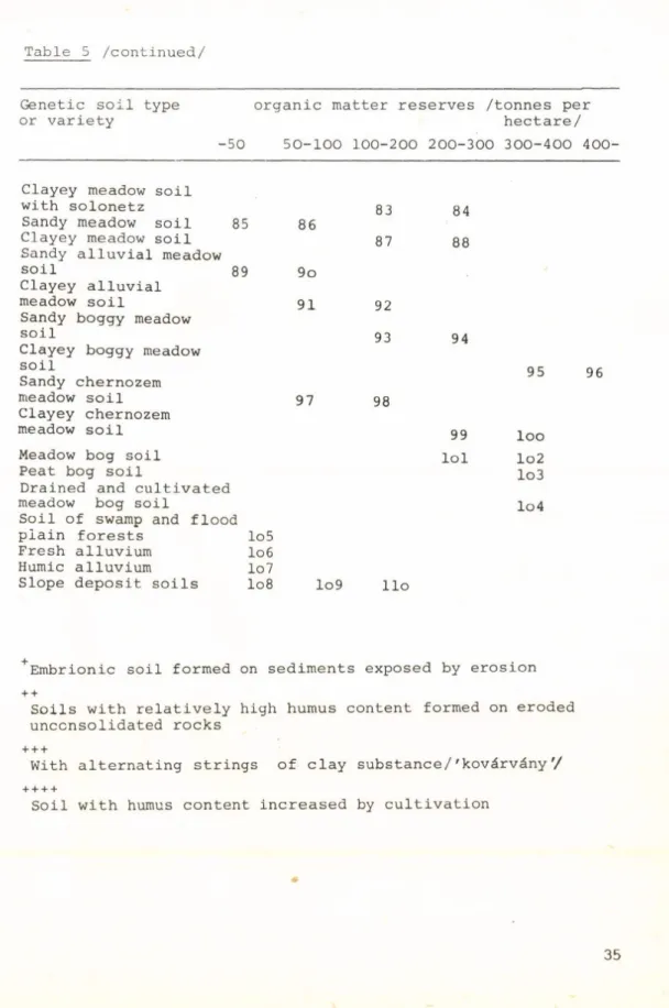
are, in many respect, the repetition of each other. If all were equally incorporated in the assessment, certain soil properties would appear multifold in the end product and, thus multiple assessment, a major danger of assessment methods, cannot be avoided. Each of the properties should be taken into consideration only once unless they are evaluated from different viewpoints (e.g. soil texture for root development or capillary water motion). The soil factors are coded as shown in Tables 5-9.

(35)

Fig. 4 Frequency of climatic year types for Komárom county and for Hungary (After LÁNG, I. - CSETE, L. - HARNOS, Zs. 1983).

1 - climatic year type; 2 = precipitation of the growing season (mm); 3 = temperature total of the growing season (°C); 4 = frequency of climatic year type (%)

In the first place the genetic soil types and humus con

ditions are included among the pedological factors. The first attaches a dynamic character to the data base since the genetic typology of soils in Hungary (STEFANOVITS, P. 1981) is founded on the presence and intensity of soil forming processes. Humus conditions comprise the depth of humus layer (in cm) and per

centage humus content. The generally applied handbook of soil survey (SZABOLCS, I. ed. 1966) defines categories for the depth of humus layer (shallow, medium or deep) and for humus content

(36)

Table 5 Coding table for factor III.17 /Genetic soil type and organic matter reserves/

Genetic soil type organic matter reserves /tonnes per

or variety hectare/

-5o 5o-loo loo-2oo 2oo-3oo 3oo-4oo 4oo- Skeletal soils with

stones or boulders Skeletal soils with

1

gravels 2

Barren earth' 3

Blown sand soils 4 Humic sand soils ++ 5

Humus carbonate'soils 6

Rendzinas 7 8 9 lo 11