Data-driven Identification of Stochastic Model Parameters and State Variables: Application to the
Study of Cardiac Beat-to-beat Variability
David Adolfo Sampedro-Puente, Jesus Fernandez-Bes, L´aszl´o Vir´ag, Andr´as Varr´o, and Esther Pueyo
Abstract—Objective:Enhanced spatiotemporal ventricular re- polarization variability has been associated with ventricular arrhythmias and sudden cardiac death, but the involved me- chanisms remain elusive. In this work a methodology for esti- mation of parameters and state variables of stochastic human ventricular cell models from input voltage data is proposed for investigation of repolarization variability.Methods:The proposed methodology formulates state-space representations based on developed stochastic cell models and uses the Unscented Kalman Filter (UKF) to perform joint parameter and state estimation.
Evaluation over synthetic and experimental data is presented.
Results:Results on synthetically generated data show the ability of the methodology to: 1) filter out measurement noise from action potential (AP) traces; 2) identify model parameters and state variables from each of those individual AP traces, thus allowing robust characterization of cell-to-cell variability; and 3) replicate statistical population’s distributions of input AP- based markers, including dynamic markers quantifying beat-to- beat variability. Application onto experimental data demonstrates the ability of the methodology to match input AP traces while concomitantly inferring the characteristics of underlying stochas- tic cell models. Conclusion: A novel methodology is presented for estimation of parameters and hidden variables of stochastic cardiac computational models, with the advantage of providing a one-to-one match between each individual AP trace and a corresponding set of model characteristics. Significance: The proposed methodology can greatly help in the characterization of temporal (beat-to-beat) and spatial (cell-to-cell) variability in human ventricular repolarization and in ascertaining the corresponding underlying mechanisms, particularly in scenarios with limited available experimental data.
Index Terms—Cardiac Electrophysiological Models, Beat-to- Beat Variability, Parameter Estimation, Joint Estimation, Un- scented Kalman Filter.
I. INTRODUCTION
B
EAT-TO-BEAT and cell-to-cell variability in ventricular electrophysiology has been well documented, this beingD. A. Sampedro-Puente, J. Fernandez-Bes, and E. Pueyo are with CIBER- BBN, Zaragoza, Spain, and with BSICoS group, I3A, IIS Arag´on, University of Zaragoza, Zaragoza, Spain (correspondence e-mail: sampedro@unizar.es).
Andr´as Varr´o and L´aszl´o Vir´ag are with the Department of Pharmacology and Pharmacotherapy, Univesity of Szeged, Szeged, Hungary. Andr´as Varr´o is with the MTA-SZTE Research Group of Cardiovascular Pharmacology, Hungarian Academy of Cardiovascular Sciences, Szeged, Hungary. This work was supported by the European Research Council through grant ERC-2014- StG 638284, by MINECO (Spain) through project DPI2016-75458-R, by MULTITOOLS2HEART-ISCIII, by Gobierno de Arag´on (Reference Group BSICoS T39-17R) cofunded by FEDER 2014-2020, by European Social Fund (EU) and Gobierno de Arag´on through a personal predoctoral grant to D.A.
Sampedro-Puente, and by projects NKFI-K119992 and NKFI-GINOP-2.3.2- 15-2016-00048, Hungary. Computations were performed by ICTS NANBIO- SIS (HPC Unit at University of Zaragoza).
an important contributor to cardiac electrical function [1], [2], [3], [4], [5]. Enhanced levels of spatiotemporal variability in ventricular repolarization have shown value to assess cardio- toxic drug effects and to identify individuals at high arrhythmic risk [6], [7], [8], [9], among others.
Temporal (beat-to-beat) variability in cellular ventricular electrophysiology has been associated with randomness in ion channel gating and variations in intracellular calcium handling [10], [11], [12], [13], [14], [15], [16]. On the other hand, spatial (cell-to-cell) variability has been suggested to be at least partly mediated by differential ionic contributions to the electrophysiology of individual cells [10], [11], [17], [18]. In this regard, the effect of variations in ion channel numbers to differences across cells has been well established, while that of variations in other characteristics related to ionic activation or inactivation is less clear [19], [20]. Computational modeling and simulation has greatly helped to shed light on the me- chanisms underlying cardiac electrophysiological variability and its ability to predict arrhythmic risk in different settings [10], [11], [19]. Specifically, computational approaches have been developed to investigate experimentally observed cell- to-cell electrophysiological differences [11], [21], [22], [23], [24] and/or beat-to-beat action potential (AP) variations, the latter after including stochasticity in modeled ionic currents [4], [11], [12], [13], [24]. Despite these advances, there is still limited understanding of the causes and consequences of ventricular repolarization variability, particularly in humans, where the less availability of data has hampered its research.
The most commonly available experimental measurement in ventricular cells is transmembrane potential. Identification of individual characteristics of underlying AP models, in- cluding estimation of model parameters and state variables, from available voltage measurements would allow characte- rization of temporal and spatial variability without the need of performing additional unaffordable experiments, which would at most provide partial descriptions of some model parameters/variables. In the present work, similarly to other modeling works [25], [26], the estimated model parameters are maximal ionic current conductances, whose variations have been established to have a major impact on both temporal and spatial variability. This estimation problem has been addressed in the literature by using a variety of methods, even if typically considering deterministic rather than stochastic cell models, thus only aiming at tackling cell-to-cell variability while not targeting representation of beat-to-beat variability, which is an important focus of the present work. As an example,
approaches based on the construction of populations of models calibrated according to experimentally measured ranges [4], [23] or distributions [20], [26] of AP-derived markers or based on emulation [27] have been proposed. These approaches provide a set of model parameter estimates for a whole population of cells, but do not provide robust identification of model parameters for each cell individually. The method proposed in this study works on an individual cell basis and uses the whole transmembrane voltage recording, comprising several APs rather than a single AP from a unique beat, as an input for the estimation, which is expected to provide more accurate representations of experimental measurement distributions even if at higher computational cost. In ven- tricular electrophysiology research, and yet more notably in humans, available experimental data is scarce, thus making this individual cell-based identification a feasible approach.
In [25], [28], a Markov Chain Monte Carlo (MCMC) method was proposed to estimate the ionic conductances of AP models directly from voltage traces as well. Our methodology, which departs from the hypothesis that model parameter and variable estimation can benefit from taking into account beat-to-beat variations in voltage signals, involves lower computational complexity than the one in [25], [28] and additionally provides an estimation of hidden states together with model parameters.
Other approaches using optimization methods like Genetic Algorithms [29] or Moment Matching [26] have also been considered for estimation of model parameters, but not state variables, from transmembrane voltage measurements. Impor- tantly, none of the above cited schemes deals with stochastic models to account for beat-to-beat AP variability, as does the methodology proposed in the present study. In the case of the optimization-based methods, the sequential nature of the AP data is sometimes not even considered but all samples are pooled together when solving the optimization problem [29].
Furthermore, these optimization-based methods do not always offer uncertainty measurements for the estimations, as can be obtained with our proposed methodology or with the method proposed in [25], [28]. As a conclusion, this work is, to the best of our knowledge, the first one providing individual cell- based identification of cardiac model parameters and variables while accounting for temporal AP variability.
The methodology here proposed is based on formulating the identification problem by means of a nonlinear state- space representation [30] and using the Unscented Kalman Filter (UKF) [31] to infer the parameters and non-measured dynamic state variables of an underlying human ventricular AP model. In this study a stochastic version of the O’Hara et al. (ORd) AP model [32] was developed and used as a basis for our state-space representations. The employed UKF filter, framed within the family of Sigma-Point filters [33], offers a probabilistic inference method to estimate the hidden variables of a non-linear system in a consistent and online manner. This constitutes a very powerful tool to reproduce both steady-state and dynamic characteristics of individual cells. Performance evaluation of the proposed methodology is carried out using sets of synthetic data generated from human ventricular AP models contaminated with different levels of noise. The methodology is subsequently tested on
experimentally measured voltage traces. Preliminary results of a more simple methodology developed based on a human ventricular phenomenological AP model were presented as a conference contribution [34].
II. MATERIALS ANDMETHODS
A. Notation
Lowercase normal letters were used to denote scalar quan- tities, lowercase boldface letters to denote column vectors and uppercase boldface letters to denote matrices. Those quantities that are time-varying are written as x(t)for continuous time andx(k)for discrete time. The notationT denotes matrix and vector transpose.
B. Human ventricular stochastic AP models
Stochastic AP models were built based on the ORd human ventricular epicardial model [32]. The ordinary differential equations representing ion channel gating were converted into reflected stochastic differential equations, following the approach presented in [4], [35]. This allowed physiologically realistic representation of stochastic ionic gating fluctuations contributing to beat-to-beat AP variability. Let vector s(t) denote the proportion of ion channels of species “s” in each state of the corresponding Markov formulation for timet. The temporal evolution ofs(t)was simulated according to:
ds(t) =As(t)dt+ 1
√Ns
ED(s(t))dw+k(t) (1) In the above equation, the first term represents the standard deterministic model of ion channel dynamics, where matrix Acontains the transition rates. The second term accounts for the stochastic fluctuations due to intrinsic noise, which was formulated using Wiener increments [4], [36]. The magnitude of this second term is inversely proportional to the square root of the number of ion channels of species “s” in the cell denoted by Ns, following the derivation of [4], [36]. The third term, k(t), represents the projection that serves to ensure that s(t) remains in the probability simplex [37], as described in [35].
Stochasticity was included in the ionic gating of four different currents, namely IKs, IKr, Ito and ICaL, which are major currents active during AP repolarization [4], [25], [38]. Following the derivations of [4], [35], matrices A, E (stoichiometry) and D (containing the rate of each transition as a function of s) in equation (1) for the stochastic ORd model were calculated as described in the following. For ionic currents defined by one ionic gate r in the ORd model, the possible channel states are open and closed. The vector s of the proportions of channels in each state is s= [r1, r0]T:
α β
r r
r
0r
1where the transition rates αr andβr are defined by:
αr= r∞ τr
(2) βr= 1
τr −αr (3)
with r∞ and τr defined as in the ORd model. Letting the proportion of channels in the open and closed states be denoted by r1 and r0, respectively, the matrices D, E and A in the Markov formulation are as follows:
D=√2
r0·αr+r1·βr
E= 1
−1
A=
−βr αr
βr −αr
This scheme with only one ionic gate, and thus two different channel states, was used for each of the fast and slow IKr
currents that are weighted averaged to obtain theIKr current.
For ionic currents defined by the product of two ionic gates r and s in the ORd model, there are four possible channel states. The vector of proportions of channels in those states is s = [r1s1, r0s1, r1s0, r0s0]T, with transition rates αr, βr, αs andβsdefined analogously to those reported in the above paragraph:
α β α β α
sβ
sr r
r r
α
sβ
sr
0s
0r
1s
0r
0s
1r
1s
1Letting the proportion of channels in each of the four states be denoted by:
• r0s0: proportion of channels in the state with the two gatesrandsclosed.
• r1s0: proportion of channels in the state with ther gate open and the sgate closed.
• r0s1: proportion of channels in the state with ther gate closed and the sgate open.
• r1s1: proportion of channels in the state with the two gatesrandsopen.
the matrices D, E andA in the Markov formulation are as follows:
D=diag
√2
r0s1·αr+r1s1·βr
√2
r0s0·αr+r1s0·βr
√2
r1s0·αs+r1s1·βs
√2
r0s0·αs+r0s1·βs
!
E=
1 0 1 0
−1 0 0 1
0 1 −1 0
0 −1 0 −1
A=
−(βr+βs) αr αs 0
βr −(αr+βs) 0 αs
βs 0 −(αs+βr) αr
0 βs βr −(αr+αs)
This scheme with two ionic gates, and four channel states, was used forIKsandItocurrents. In particular, in the case of Ito, the total current was decomposed as a weighted average of four individual currents, each of which represented by the
product of two ionic gates: a·ifast, a·islow, aCaMK·iCaMK,fast andaCaMK·iCaMK,slow.
ForICaL, ordinary differential equations representing gating variables were converted into stochastic differential equations following the subunit-based approach used in [11]. For a gating variablexs, the evolution of the probability of this gate being open was calculated as:
dxs(t) = xs∞−xs τs
dt+
pxs∞+ (1−2xs∞)xs
√τs·Ns
dw (4) The number of channels Ns of each ionic species “s” was computed as follows. For IKs, IKr and Ito, experimentally measured unitary current values were available and were used to calculate Ns as the maximum conductance of ion channel
“s” in the ORd model, denoted byGs, divided by the unitary conductance of ion channel “s”, denoted by gs. Values forgs were taken from [11], [39], [40] and adjusted for temperature and/or extracellular potassium concentration following [41], [42]. For ICaL, the number of channels was computed by dividing the maximum ICaL current by the single-channel current iCaL times the channel opening probability. Table I shows the values used in the computations for the default ORd model.
TABLE I
NUMBER OF CHANNELS FORIKs,IKr,ItoANDICaL
IKs IKr Ito ICaL
Ns 169 3621 606 20121
C. State-space formulation
State-space representations were formulated to describe non-stationary stochastic processes with measured and hid- den variables [30]. Specifically, the stochastic ORd model, described in section II-B, but with unknown ionic current conductances, was casted into a non-linear discrete-time state- space model, following numerical integration with the Euler- Maruyama method. As an example, equation (1) for vector s(t)was written in the form:
s(k) =s(k−1) +As(k−1)∆t + 1
√NsED(s(k−1))dw+k(k−1) (5) wherekis a discrete index (k∈N),∆tis the integration time step (constant in this study) anddwis a vector of independent Wiener increments sampled from a Gaussian distribution with zero mean and variance equal to ∆t. The overall state-space representation was described by the following two equations:
x(k) = f(x(k−1),q(k−1),θ) (6) y(k) = h(x(k)) +r(k). (7) Equation (6), called the process or transition equation, collects the discretized set of differential equations that define the state variables of the stochastic ORd model, stacked in vector x(k), thus including the equations that model the temporal evolution of transmembrane voltage, intracellular ion
concentrations and proportion of channels in each state for each ionic species. The non-linear function f(·) in equation (6) has three input vectors, namely the vectorx(k)of model state variables, the vectorq(k)of non-additive process noises (related to the Wiener increments) described in II-B and the vectorθof model parameters. The components of vectorq(k) take values sampled from independent Gaussian distributions with zero mean and variance equal to∆tfor such components corresponding to the stochastic gating variables and zero for all other components.
The ORd model was parametrized with factors multi- plying the conductances of the following ionic currents [26]: slow delayed rectifier potassium current, IKs; rapid delayed rectifier potassium current, IKr; transient outward potassium current, Ito; L-type calcium current, ICaL; in- ward rectifier potassium current, IK1; and sodium current, IN a. Hence, the vector of static model parameters, θ = {θKs, θKr, θto, θCaL, θK1, θN a}, represents variations in the ionic conductances ofIKs,IKr,Ito,ICaL,IK1 andIN a rel- ative to the default values in the ORd model,Ij =Ij,ORd·θj. Note that the same factor θj applies to the number of ion channels of each species (Table I): Nj =Nj,ORd·θj, as the unitary conductance of each ionic species was assumed to be constant based on previously reported experimental findings [43]. The values of the parameters inθwere inferred for each input AP trace.
In equation (7), called the measurement equation,y(k)is the measured variable (transmembrane voltage), which is defined as y(k) = v(k) +r(k), where v(k) represents the noiseless transmembrane potential andr(k) is additive white Gaussian noise. Hence, the function h(·) in equation (7) is linear, as it takes only the component of x(k) corresponding to the transmembrane voltage,v(k).
D. Augmented state-space
A state augmentation approach [30] was used to jointly estimate the parameters and state variables of the stochastic ORd model for a given input (synthetic or experimental) AP trace. Following the notation introduced in II-C, the static parameters in vector θ were replaced with a new vector of time-varying variablesθ(k)e using a random walk model with drift:
θ(k) =e θ(ke −1) +δ(k). (8) where the components of the artificial noiseδ(k)introduced in the definition ofθ(k)e dynamics are i.i.d. zero-mean Gaussian processes with very small variance. This artificial noise allows adapting the parameter values in an online manner while the input AP trace is being filtered and can be given an interpretation similar to the small constant step size in adaptive filtering theory [44]. In this work, this artificial noise had the same variance,σ2θ, for all six individual parameters.
In addition to the augmentation due to the inclusion of the parameters as additional state variables, the noise process q(k) was also incorporated as part of the augmented state space. This is a standard approach for estimation when dealing with non-additive noise processes (see e.g. [30, Chap. 5]).
By stacking the vector x(k) of model state variables, the
new vector θ(k)e of model parameters and the vector q(k) of process noises, a new “augmented” state vector z(k) was defined as:
z(k) =h
x(k),q(k),θ(k)e iT
(9) The resulting state-space model has the following formulation:
z(k) = fa(z(k−1)) +(k) (10) y(k) = ha(z(k)) +r(k) (11) where fa and ha are the augmented versions of f and h from equations (6) and (7). The vector (k) contains two types of noises, those associated with the Wiener increments of the stochastic model (accounted for by q(k)) and those associated with the new parameter vector θ(k)e (accounted for by δ(k)). The components in vector (k) corresponding to the original state variables x(k) take a value of zero, while the rest of components are zero-mean Gaussian noises with variance equal to the integration time step, ∆t, for the components corresponding to q(k) and variance equal to σ2θ for the components corresponding to θ(k).e
E. UKF-based joint state and parameter estimation
As the state-space representation defined in equations (10) and (11) is nonlinear, the Unscented Kalman Filter (UKF) [31] was used for state and parameter inference. UKF is based on approximating the posterior distributionp(z(k)|y1:k), with y1:k denoting all the samples up to time k of the measured variable y, by using a deterministic set of suitably chosen points called Sigma Points. UKF has shown better performance than the Extended Kalman Filter (EKF) at a comparable computational cost [45]. Also, UKF involves much lower computational cost than Monte Carlo-based methods, like Particle Filters[30].
A scheme of the proposed methodology is shown in Fig.
1. A noisy (synthetic or experimental) AP trace is provided as an input for UKF to infer the evolution of a set of state variables (transmembrane voltage, ionic concentrations and ion channel states) and model parameters (ionic current conductance factors) based on the state-space representation described in equations (10) and (11).
Being L the dimension of this state-space representation, 2L+ 1Sigma Pointswere deterministically generated for each time step. These Sigma Points were propagated through the model transition function fa(·) and used to approximate the posterior mean and covariance according to the so called Un- scented Transform [31]. Since the dimension of z(k) was 95 (56 state variables, 33 process noises and 6 model parameters), 191 Sigma Pointswere computed.
For the estimation process, two free hyper-parameters re- quired prior definition: the process noise variance σθ2 related to model parameter estimation and the measurement noise variance σ2r. The practical selection of these parameters is not trivial and its effects are explored for different scenarios in Section III. In addition, the UKF algorithm has three parameters, namely α, β and κ, which in this study were assigned the following values: α = 1, β = 0, κ = 3−L, as in [34].
Fig. 1. Scheme of the proposed methodology. A noisy AP trace is the input to a model-based filtering algorithm. This AP may have been synthetically generated using a computational AP model or experimentally recorded. The filtering algorithm outputs a filtered (noiseless) AP and a set of estimated hidden states and model parameters for a computational AP model used as a basis for the study (ORd model in this study). New AP traces can be computed from the estimated model under different simulation conditions.
In the following the notation aˆ was used to denote the estimate of a generic variablea. Analogously, ˆa(k)was used for a time-varying estimate. When in the following a unique estimated value, e.g. for the parameter vectorθ, is provided, the average of the estimated values over the lastN = 5cycles was considered, as using a larger number of cycles did not render improved estimation performance.
F. Synthetic Data
A set of AP models was built based on the ORd human ventricular epicardial model [32]. Each AP model in the dataset was obtained by varying the conductances defined as parameters of the model:IKs,IKr,Ito,ICaL,IK1, andIN a. These models aimed to represent inter-cellular variability and were used to validate the presented methodology.
A total of 500 models were initially generated by sampling the nominal conductance values of the ORd model in the range ±100% using the Latin Hypercube Sampling method [4], [23], [46]. Out of all generated models, only those satisfying the calibration criteria shown in Table II were retained. Such criteria were based on experimentally available human ventricular measures of steady-state AP characteristics [32], [47], [48], [49], [50]. These characteristics included:
APD90|50, denoting 1 Hz steady-state AP duration (APD) at 90%|50% repolarization (expressed in ms); RMP, standing for resting membrane potential (in mV); Vpeak, measuring peak membrane potential following stimulation (in mV); and
∆APD90, which was calculated as the percentage of change in APD90 with respect to baseline when selectively blocking IKs,IKr or IK1 currents (measured in ms). For some of the above characteristics, only experimental values of the mean and standard error of the mean, rather than minimum and maximum limits, were available. In those cases, limits were defined by mean±three calculated standard deviations, as this would cover 99% of the measurements if the data followed a normal distribution. After applying the described calibration criteria, the initial set of 500 models was reduced to a set of
131 selected models.
TABLE II
CALIBRATION CRITERIA APPLIED ONTO HUMAN VENTRICULAR CELL MODELS.
AP characteristic Min. acceptable value Max. acceptable value Under baseline conditions ([32], [47], [48])
APD90(ms) 178.1 442.7
APD50(ms) 106.6 349.4
RMP (mV) -94.4 -78.5
Vpeak(mV) 7.3 -
Under 90%IKsblock ([32])
∆APD90(%) -54.4 62
Under 70%IKrblock ([49])
∆APD90(%) 34.25 91.94
Under 50%IK1block ([50])
∆APD90(%) -5.26 14.86
In each model of this synthetic dataset, the variation in the conductances of the four stochastic ionic currents with respect to the default ORd model was correspondent with a proportional variation in the number of ion channels (used in the stochastic term of the differential equations).
In addition to this synthetic dataset generated with the ORd model, additional AP traces were generated with a stochastic version of the ten Tusscher-Panfilov (TP06) epicardial AP model [51]. Those additional AP traces were used to test the performance of our proposed methodology over data obtained from a different human ventricular cell model.
Trains of 550 beats paced at a frequency of 1 Hz were simulated by using the Euler-Maruyama scheme with an integration time step of dt = 0.02 ms. The stimulus current was a1-ms duration rectangular pulse of52-pA/pF amplitude.
Only the last 50 simulated beats were used as input signals to the estimation methodology to guarantee that steady-state had been reached. Gaussian noise, denoted byr(t), with zero mean and noise varianceσr2was added to the simulated mem- brane potential to account for noise present in experimental recordings. The effect on the estimation results of varying the values of σr to represent different signal-to-noise ratios (SNRs) was analyzed.
G. Experimental data
Two ten-second AP recordings acquired using conventional microelectrode techniques in trabecular preparations from right ventricles of undiseased human donor hearts, as described in [32], were available for this study. The recordings were obtained from previous studies, with tissue preparations having been donated for research in compliance with the Declaration of Helsinki and approved by the Scientific and Research Ethical Committee of the Medical Scientific Board of the Hungarian Ministry of Health (ETT-TUKEB), under ethical approval No 4991-0/2010-1018EKU (339/PI/010). Pacing fre- quency was 1 Hz. Each AP trace was linearly interpolated to a sampling interval of 0.02 ms and was replicated five times. The resulting 50-cycle trace was fed as an input to the estimation algorithm to ensure convergence to stable values for the last analyzed replication.
H. Methodology assessment
The proposed methodology was assessed as follows:
1) Noisy AP filtering capability: For synthetic data, the root mean square errorξv between the original noiseless AP trace, v(k), and the estimated AP trace, v(k), was calculated overˆ the lastN = 5 simulated cycles:
ξv= v u u t
1 KN
KN−1
X
k=0
|v(k)−v(k)|ˆ 2, (12) whereKN is the number of samples contained within the last N = 5cycles.
2) State and parameter estimation: For the synthetic dataset generated with the ORd model, estimates of model pa- rameters (i.e. factors multiplying maximal ionic conductances) and hidden states (i.e. model state variables) computed using the proposed methodology were compared with the original values used to generate the synthetic input AP traces. The mean relative error (ηzj) between the actual and estimated values of each state variable was calculated over the last N = 5simulated cycles:
ηzj = 1 KN
KN−1
X
k=0
|zj(k)−zˆj(k)|
|zj(k)|
, (13)
wherezj is the actual value of the state variable j and zˆj is the estimated value, withj= 1,· · ·, L, beingLthe length of the augmented state vector z(k). The mean relative error ηzj
in the estimation of each model parameterzj was analogously calculated.
A global accuracy measurement of model parameter esti- mation was defined as the average of the mean relative errors (adimensional by definition) for all estimated parameters:
¯ ηθ= 1
M X
θ0∈θ
ηθ0, (14)
whereηθ0 is the mean relative error for model parameterθ0 ∈ θ andM = 6 (the number of estimated model parameters).
3) Reproducibility of AP markers: For both synthetic and experimental data, the performance of the proposed metho- dology was additionally assessed by comparing AP-derived markers from input and estimated AP traces. Specifically, given an input AP trace, estimates of the stochastic ORd model parameters were computed using the proposed methodology and that estimated model was then simulated to generate new AP traces from which AP-derived markers were computed.
The following steady-state and temporal variability mea- surements of repolarization were calculated over those input and simulated AP traces:
• Average of APD at 90% repolarization (APD90) over the lastN = 30cycles:
mAPD90 = 1 N
N
X
n=1
APD90(n), (15) and standard deviation of APD90 over the last N = 30 cycles:
sAPD90 = v u u t
1 N−1
N
X
n=1
(APD90(n)−mAPD90)2, (16)
0 200 400
-100 -50 0 50
0 200 400
-100 -50 0 50
(a)σr= 0.25mV (b) σr= 10mV
Fig. 2. Last cycle of AP traces: In black, the synthetic noiseless AP trace generated by the original ORd model; in blue line, the noisy version of that AP,y(k), which is used as input to our proposed method with two different values for the standard deviation of the measurement noise, σr; in red, the mean estimated voltage at each time instant, denoted byx; and in grey, the¯ estimated uncertainty bands, i. e.,x¯±3σx(withσxdenoting the estimated standard deviation of voltage).
• Short-Term Variability (ST V) of APD90, defined as the average distance perpendicular to the identity line in the Poincar´e plot, computed for the lastN = 30 cycles as:
ST V =
N−1
X
n=1
|APD90(n+ 1)−APD90(n)|
(N−1)√
2 , (17)
III. RESULTS
A. Noisy AP filtering
The proposed methodology was able to filter out the mea- surement noise in input AP signals even in cases of low SNR.
Fig. 2 presents the last cycle of a synthetic noiseless AP trace generated with the stochastic ORd model on top of two noisy APs obtained by adding Gaussian noises with zero mean and standard deviation values of σr = 0.25 mV and σr = 10 mV, respectively, and the filtered APs output by our proposed methodology assuming the level of measurement noise was known. In this figure, as well as in all subsequent figures, x¯ denotes the mean estimated value of the represented variable and σx, the estimated standard deviation. For both levels of noise, the methodology (with σθ = 10−12) was able to accurately estimate the synthetic noiseless AP, thus rendering it useful to evaluate AP markers from noisy AP traces as those obtained from experimental recordings.
In Table III, root mean square error values ξv calculated according to equation (12) for the two different SNR levels are presented. As can be observed, our method was able to almost entirely reduce the noise in the input AP traces even for a high level of measurement noise.
TABLE III
ξvROOTMEANSQUAREERROR(MV)INAPFILTERING σr (mV) 0.25 10
ξv(mV) 0.0160 0.1429
10-2 10-1 100 101 102 10-2
10-1 100
r = 0.25mV r = 10mV
Fig. 3. Root mean square errorξvin AP filtering for different actual (σr) and estimated (σbr) levels of measurement noise.
B. Sensitivity of the methodology with respect to its own parameters
When the level of measurement noise is unknown, the value ofσrneeds to be set according to some criteria. While under homoscedastic conditionsσrcould be readily estimated during the resting phase of the AP, such an estimation might be poor under other conditions. In Fig. 3 assessment of the sensitivity of our proposed methodology with respect to the estimated value ofσris presented. Specifically, the effect of varying the estimated measurement noise,σbr, on the errorξv is presented for two different levels of noise added to input AP traces generated with the stochastic ORd model, being these two levels correspondent with σr = 0.25 mV and σr = 10 mV.
As can be observed from the figure, in both cases there was a broad range ofσbr values with similarly good performance in terms of AP filtering (note the log-scale for the x-axis).
An apparently counter-intuitive result is that the optimal value ofbσr did not exactly match the value ofσr, but it was slightly higher. This may be explained because bσr accounts not only for measurement noise but also for model misspecifi- cation. Under high SNR (lowσr), this misspecification, which could be due to small errors in model parameter estimation, can be comparable to the input noise.
Regarding the sensitivity of the methodology with respect to σθ, Fig. 4(a) shows that varyingσθ did not significantly affect the error in AP filtering. However, it more notably affected the error in parameter estimation, particularly when very small or very largeσθ values were used, as shown in Fig 4(b).
In particular, the estimation errorηθwas increased for very small values ofσθdue to lack of convergence in the estimation for 50 simulated APs. For very large σθ values (≥10−6),ηθ was increased due to the algorithm being stuck in local minima where its performance was not satisfactory and could not be improved in any direction or due to notable oscillations around the mean estimated value. Consequently, the selection of the value forσθwas deemed to be important to obtain an accurate model parameter estimation.
According to the results shown in Fig. 3 and Fig. 4,σθ = 10−12 was selected and all results presented in the following Sections III-C and III-D correspond to that value, while the measurement noise variance was taken asσbr=σr.
C. Estimation of model parameters and hidden states The proposed methodology was able to additionally esti- mate hidden states from a given input AP trace according to
(a)
10-14 10-12 10-10 10-8 10-6
0.018 0.02 0.022
(b)
10-14 10-12 10-10 10-8 10-6
100
Fig. 4. Root mean square errorξvin AP filtering (a) and average of mean relative parameter estimation errors η¯θ (b) evaluated for different levels of σθ.
0 500 1000 1500
time (ms) 0
0.5 1
X Krf
0 500 1000 1500
time (ms) 0
0.05 0.1 0.15 X Ks
Fig. 5. Open probabilityXKrfofIKr(top panel) and open probabilityXKs
ofIKs (bottom panel). The value in the stochastic ORd model is shown in blue, while estimated mean (¯x) and uncertainty bands (¯x±3σx) are shown in red and grey, respectively.
the stochastic model described by fa(·) in equation (10). In particular, for the case of input AP traces being synthetically generated using the stochastic ORd model, a comparison could be established between actual and estimated values of model parameters and hidden states.
Fig. 5 illustrates the input and estimated (mean ± three standard deviations) proportions of open channels for IKr
and IKs in the last two simulated cycles. The proposed methodology was not only able to track the mean value of the state variables describing the proportions of open channels at each time instant but also provided uncertainty ranges, which were larger forIKs than for IKr.
Fig. 6 illustrates the estimated (mean ± three standard deviations) model parameters along 50 simulated cycles. The mean estimated values converged to the input value in less than 40 cycles. Uncertainty ranges in the estimation were provided as well.
Results of model parameter estimation for the population of 131 stochastic AP models described in Section II-F are
0 20 40 time (s) 0
0.5 1 1.5
Ks
0 20 40
time (s) 0
0.5 1
Kr
0 20 40
time (s) 0
0.5 1
to
0 20 40
time (s) 0
0.5 1
CaL
0 20 40
time (s) 0
0.5 1 1.5
K1
0 20 40
time (s) 0
0.5 1
Na
Fig. 6. Estimation of model parameters. Mean estimates (¯x) are shown in red and uncertainty bands (¯x±3σx), in grey.
Fig. 7. Mean relative errorηθ0 for each of the estimated model parameters over a population of 131 stochastic AP models.
presented in Fig. 7. As can be observed, the estimation accuracy was very high for most parameters in the majority of tested models. The maximum relative errorηθ0 was obtained forθKs due to the almost negligible effect of its variations on the baseline AP.
D. Estimation of AP markers
In this section the performance of the proposed methodo- logy is evaluated in terms of its ability to replicate input AP traces and AP-derived markers. Fig. 8 shows the statistical distributions of mAP D90 and ST V over the population of stochastic cell models described in Section II-F, calculated from both actual and estimated APs. A very good match was observed between both distributions for each of the two AP markers.
Additionally, the accuracy of the proposed methodology to reproduce AP markers measured from synthetic data was tested over APs generated with a different human ventricular cell model, namely a stochastic version of the TP06 model [51]. Fig. 9 (top panel) shows input APs generated with the stochastic TP06 model, APs estimated with the proposed methodology as well as APs generated with the default ORd model (used as a basis for the proposed methodology) for
0 200 400 600 800 0
2 4 6
Density
10-3
Input Estimated
0 10 20
0 0.1 0.2 0.3
Density
Fig. 8. Statistical distributions over a population of 131 AP models of (left) mAPD90and (right)ST V calculated from actual APs in blue and estimated APs in red.
0 200 400 600 800 1000 1200 1400 1600 time (ms)
-100 -50 0 50
V (mV)
Input, TP06 - Epi Estimated ORd - Epi
0 10 20 30 40 50
cycles 220
240 260 280 300 320
APD (ms)
Input, TP06 - Epi Estimated ORd - Epi
Fig. 9. AP traces over 2 simulated cycles (top panel) and APD time series over 50 simulated cycles (bottom panel) generated with the stochastic TP06 model (in blue), estimated with the proposed methodology (dashed red) and generated with the stochastic default ORd model (black).
comparison. Intrinsic differences between the ORd and TP06 models (e.g. the TP06 model produces a much more square AP) may explain the lack of complete match between input and estimated APs. In terms of the root mean square errorξv, this took a value of 6.96 mV for our proposed methodology versus 22.89mV for the reference ORd model.
In addition, Fig. 9 (bottom panel) presents corresponding APD time series over 50 simulated cycles calculated for APs computed from the stochastic TP06 model, the proposed methodology and the default stochastic ORd model. The match between input and estimated APDs was very good, with a mean absolute error of 0.16 ms between average APDs, while such an error was of 71.68 ms for the default ORd model.
Beat-to-beat variability was, however, larger for the input data generated with the TP06 model than for the estimated data or the data generated with the default ORd model (STV being 3.42 ms, 1.69 ms and 1.89 ms, respectively).
E. Application onto experimental data
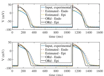
Application of the proposed methodology onto experi- mentally recorded input AP signals is illustrated in Fig.10.
The value for the algorithmic parameter σθ was selected by searching for in the range between 10−15 to10−6. The best results were obtained for10−7, which is the value used for the results presented in the following. Also, the valueσr= 1mV
was set. Of note, when applying our proposed methodology onto experimental data, which presents AP shapes different from the one of the default ORd model, issues regarding the estimation algorithm being stuck in local minima are more common. For that reason, the choice of the value for σθ is especially important, as too large or too small values might lead to estimated models not generating valid AP traces.
In this section, methodological performance is evaluated by comparing experimental AP traces and AP traces build from the parameterized ORd model with the parameter va- lues estimated by our proposed approach. Our methodology departed from the default ORd model (for both epicardial and endocardial cells) and refined it to best fit the input AP trace.
A satisfactory match was found between input and estimated APs, with some differences in the plateau and resting phases, but with good overall agreement and very close AP durations.
APs generated with the default epicardial and endocardial ORd models are shown for comparison.
Table IV shows the root mean square errors ξv obtained in the estimation from experimental human AP traces, while Table V shows the estimated parameter values. As can be noted, the estimation errors obtained by our methodology for the two human AP traces were clearly lower than those obtained with epicardial and endocardial ORd models.
The performance of the proposed methodology was in this case not evaluated in terms of variability measurements, as simulated APs corresponded to single cells whereas experi- mental AP traces were recorded in tissue, where electrotonic coupling notably mitigates the effects of ionic current fluctu- ations contributing to beat-to-beat variability.
TABLE IV
ξvROOTMEANSQUAREERROR(MV)IN FITTING EXPERIMENTALAP TRACES
(mV) AP trace 1 (mV) AP trace 2 ξv(This Method - Endo) 8.2432 6.3393
ξv(ORd - Endo) 11.5096 10.1043
ξv(This Method - Epi) 5.0071 10.3788
ξv(ORd - Epi) 9.0270 14.8517
IV. DISCUSSION
In this work, a novel approach based on formulation of state-space representations and the use of the Unscented Kalman Filter has been proposed as a method to estimate the non-measured state variables and parameters of ventricular nonlinear stochastic computational models. The proposed me- thodology was able to reproduce individual input AP traces and replicate statistical distributions of AP-derived markers like APD or STV. As such, the methodology can be a powerful tool to investigate the ionic mechanisms underlying
TABLE V
ESTIMATED PARAMETER VALUES FOR THE TWO EXPERIMENTALAP TRACES USING THE HUMAN VENTRICULAR ENDOCARDIALORD MODEL.
θKs θKr θto θCaL θK1 θN a
Exp. 1 1.9997 1.9996 1.9996 1.8027 0.0538 1.4840 Exp.2 0.5481 1.4217 0.7214 1.5032 1.2950 0.1368
0 200 400 600 800 1000 1200 1400 1600 time (ms)
-100 -50 0 50
V (mV)
Input, experimental Estimated - Endo Estimated - Epi ORd - Endo ORd - Epi
0 200 400 600 800 1000 1200 1400 1600 time (ms)
-100 -50 0 50
V (mV)
Input, experimental Estimated - Endo Estimated - Epi ORd - Endo ORd - Epi
Fig. 10. Experimental AP traces (blue) and estimated AP traces obtained with the proposed methodology based on stochastic versions of epicardial (dotted yellow) and endocardial (dashed red) ORd models. Default stochastic epicardial (solid black) and endocardial (dashed black) ORd models are shown as a reference. Top and bottom panels correspond to two different experimental recordings.
human ventricular AP traces and their associated beat-to-beat variability, particularly when experimental measurements are scarce, as is usually the case with human data, and previously proposed methodologies are either not applicable or present considerable limitations.
In the following, relevant characteristics of the proposed methodology as well as major benefits and shortcomings associated with its use are discussed:
a) Methodology calibration: According to the presented results, calibration of two parameters of the proposed me- thodology, σr and σθ, turns out to be important to obtain an accurate estimation. The first one, σr, accounts for both measurement noise and model-to-data mismatch, hence its calibration is relatively easy in most cases. Although, in principle, the definition of σθ should not be so straightfor- ward, our results show that a wide range of values for σθ
provide similarly good estimation performance. Specifically, our analysis on the synthetic data described in Section II-F has demonstrated that this feasible range spans several orders of magnitude. In other cases where the model adjusts poorly to the input AP trace, the optimal value for σθ can be found by sweeping over a large range of values and selecting the one leading to the best match to the input data.
b) Filtering noisy data: The proposed methodology is able to filter out the measurement noise even for AP recordings with very low SNR levels. This can be very useful to improve the accuracy in the evaluation of AP markers from experimen- tal noisy AP traces like, for instance, those measured using optical mapping techniques.
c) Identification of model parameters and hidden states:
A state-augmentation approach was used for joint state and pa- rameter estimation, considering the compromise between per- formance and computational cost. Other joint estimation tech- niques like Expectation Maximization or Rao-Blackwellization [30] introduce a large penalty in the computational cost, associated with the need to perform several passes over the
hundreds of thousands of samples of AP traces, and were thus discarded for this problem. Importantly, the probabilistic methodology presented in this study provides estimation errors for each variable along time, thus offering uncertainty mea- sures associated with the estimation process, which could be used as a basis for further Uncertainty Quantification studies (see e.g. [52]).
Our results prove to be accurate for all estimated ionic factors except for the factor related to the IKs conductance (Fig. 7). This lack of accuracy in the estimation of one of the model parameters is related to the issues of identifiability and observability, the latter possibly being in practice more difficult to satisfy [53]. Previous studies targeting estimation of neuron model parameters from voltage time series have dealt with this [54]. For the augmented state-space considered in this study, a formal identifiability / observability analysis would be of high interest.
In our case, and in line with reported experimental and simulated evidences on the lack of effects ofIKsvariations on baseline AP [49], [55], [56], the cellular ORd model used as a basis for this study led to similar AP traces for a relatively large range ofIKs conductance values and, in such scenario, the estimation algorithm may fail to identify the corresponding conductance value. Nevertheless, the intrinsic characteristics of our proposed approach provide some advantages with respect other works. Our methodology, by using stochastic models, leads to a significant reduction in parameter uncertainty as compared to other studies where a cell model is fit to only one (averaged or not) AP [57] rather than to a whole AP trace comprising several consecutive beats. The fact of including data across several beats allows integrating temporal variability information into the estimation process, thus making it more robust, as different parameter combinations might lead to comparable APs but dissimilar beat-to-beat AP variability measurements. In addition, our proposed methodology is also able to estimate model hidden states, including ionic gating characteristics and intracellular concentrations, thus facilitat- ing assessment of whether the model renders physiologically plausible outcomes. Furthermore, our Bayesian methodology explicitly delivers precision measurements for each estimated variable. When a parameter value is difficult to identify, our approach provides an associated high estimation variance, as was for instance the case forθKs (Fig. 6).
The above described uncertainty in the estimation of one of the model parameters could be classified as ‘practical unidentifiability’ according to the classification provided in [58], meaning that, by using input data obtained with a different protocol, it could be possible to increase the amount of available information for the estimation. In our case, one option would be to consider data measured at different pacing frequencies as in [25], [26], [29] or to consider combined data measured under control and following ionic inhibitions as in [26]. Future studies should address the application of the methodology proposed in this work onto AP data measured at different stimulation frequencies or under ionic inhibitions.
d) Application onto data from different origins: Our presented methodology is able to adjust a developed stochastic version of the ORd model to fit a population of input AP data
in such a way that a one-to-one correspondence is established between each individual AP and a set of model parameters underlying it. This ability has been successfully tested over a synthetic population of cellular AP data generated with the ORd model, where the proposed methodology has additionally shown to provide a robust way to approximate distributions of AP markers of interest.
For data presenting AP shapes markedly different to that of the ORd model used as a basis for the estimation, either being recorded experimentally or generated by other human ventricular computational models, our proposed methodology is still able to reproduce the corresponding AP traces. Never- theless, in those cases, some differences exist between input and estimated APs due to the fact that some specific charac- teristics of the ORd model cannot be modified by just varying maximal ionic conductances. In particular, APs generated with the TP06 model show higher beat-to-beat variability, for a comparable mean APD, than those generated with the ORd model, as shown in our results. Remarkable differences in several ionic currents between the two models, includingIKs
characteristics, may explain such a divergence in terms of beat- to-beat variability. In the case of the analyzed experimental AP traces, beat-to-beat variability measurements could not be compared between input and estimated APs, as variability observed in tissue is considerably lower than in isolated cells due to electrotonic coupling effects. Unfortunately, only human ventricular data recorded in tissue, not in isolated cells, was available for this study. Nevertheless, the proposed methodology was able to estimate the experimental AP traces, rendering similar average APDs.
To the best of our knowledge this is the first study where stochastic cell models are used as a basis for model para- meter and state variable estimation from ventricular AP data, thus aiming at providing a method to reproduce variability measurements and investigate the mechanisms behind it. In [25] a method is presented to fit different types of AP data but not to reproduce beat-to-beat variability. In [4], stochastic cell models are used but model parameters representing ionic current conductances are identified to replicate ranges of beat- to-beat variability measures only, while not necessarily the actual statistical distribution of such measures or the corre- sponding AP shapes. In other works based on the population- of-models approach, such as [20], [26], methods are developed to reproduce distributions of AP markers, but in this case without targeting beat-to-beat variability. Our approach can approximate statistical distributions of AP markers and has the additional advantage of producing a one-to-one corre- spondence between individual AP traces (and corresponding AP-based markers) and a set of parameter values for an underlying cell model. This can be of significant help to unravel ionic mechanisms involved in different investigated electrophysiological behaviors, including temporal variability.
e) Robustness analysis: Our proposed methodology is evaluated in a range of scenarios using both synthetically generated and experimentally measured AP data. In the case of synthetic input data, the ability of our approach for model parameter and state variable estimation is assessed by consi- dering different SNR and a wide range of possible parameter