agnostic approach employing Hellinger distance
Tam´as Ficsor1[0000−0002−8442−6652]and G´abor Berend1,2[0000−0002−3845−4978]
1 Institute of Informatics, University of Szeged, Hungary
2 MTA-SZTE Research Group on Artificial Intelligence {ficsort, berendg}@inf.u-szeged.hu
Abstract. Word embeddings can encode semantic and syntactic features and have achieved many recent successes in solving NLP tasks. Despite their successes, it is not trivial to directly extract lexical information out of them. In this paper, we propose a transformation of the embedding space to a more interpretable one using the Hellinger distance. We additionally suggest a distribution-agnostic approach using Kernel Density Estimation. A method is introduced to measure the interpretability of the word embeddings. Our results suggest that Hellinger based calculation gives a 1.35% improvement on average over the Bhattacharyya distance in terms of interpretability and adapts better to unknown words.
Keywords: Word Embeddings·Interpretability·Computational Semantics.
1 Introduction
There have been many successes in the field of NLP due to the application of word embeddings [3]. There is a new forefront as well called contextual embeddings (e.g., BERT), which further increases the complexity of models to gain better performance.
[2] showed there is only a small performance increase on average regard to complexity, but this performance varies on each employed task. Thus static embeddings still serve a good ground for initial investigations about the interpretability.
Prior research by [12] has investigated the issue of semantic encoding in word embeddings by assuming that the coefficients across each dimensions of the embedding space are distributed normally. This assumption may or may nor hold for a particular embedding space (e.g. the normality assumption is unlikely to hold for sparse word representations), hence we argue for the necessity of similar algorithms that operate in an distribution-agnostic manner. We introduce such a model that allows the word embedding coefficients to follow arbitrary distributions by relying on Kernel Density Estimation (KDE). A further novelty of our work is that we propose the application of the Hellinger distance – as opposed to the Bhattacharyya distance – which could be a more suitable choice due to its bounded nature. We also make our source code publicly available1in order to foster the reproducibility of our experiments.
1https://github.com/ficstamas/word_embedding_interpretability
2 Related Work
Word embeddings can capture the semantic and syntactic relationships among words [9].
[15] was one of the first providing a comparison of several word embedding methods and showed that incorporating them into established NLP pipelines can also boost their performance.
There are several ways to incorporate external knowledge into NLP models. Related methods include the application of auto-encoders [16], embedding information during training [1] or after the training phase, called retrofitting [5]. One way to understand the semantic encoding of a dimension in embedding spaces is to link them to human interpretable features. [12] introduced the SEMCAT dataset and a method that relies on the Bhattacharyya distance for doing so. Their proposed method can produce a more interpretable space where each dimension encodes a predefined semantic category from the SEMCAT dataset, which was tested on GloVe [11] word embedding. There have been various approaches to find these semantic categories. Such an approach is to construct datasets in a way which involves human participants only [8], or in a semi-automated manner where the construction is based on statistics to make the connections between the members of semantic categories and curated later by human participants [13].
Our proposed approach relies on the application of the Hellinger distance, which has already been used in NLP for constructing word embeddings [7]. Note that the way we rely on the Hellinger distance is different from prior work in that we use it for improving the interpretability of some arbitrarily trained embedding, whereas in [7] the Hellinger distance served as the basis for constructing the embeddings.
3 Our Approach
In this paper we follow a process to produce interpretable word vectors which is similar to [12]. Unlike [12], who trained their own GloVe embeddings, in order to mitigate the variability due to training, we are using the pre-trained GloVe with 6 billion token as our embedding space with 300 dimensions. Furthermore the SEMCAT dataset is going to serve as the definition of the semantic categories. Instead of GloVe and SEMCAT other kinds of embeddings (e.g., fastText) and datasets incorporating semantic relations (e.g., the McRae dataset [8]) can be integrated into our framework.
3.1 Information Encoding of Dimensions
The assumption of normality of the embedding dimensions is statistically a convenient, however, empirically not necessarily a valid approach. As the normal distribution is simple and well-understood, it is also frequently used in predictive models, however, assuming normality could have its own flaws [14]. The assumption of normality plays an essential role in the method proposed by [12], that we relax in this paper.
If we try to express the information gain from a dimension regarding some con- cept, we can do so by measuring the distance between the concept’s and dimension’s distribution. In order to investigate the semantic distribution of semantic categories
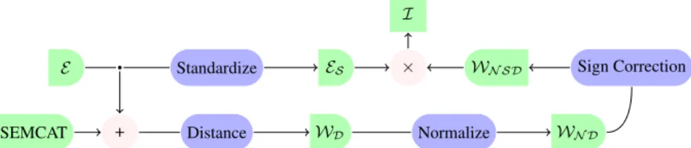
E Standardize ES
SEMCAT + Distance WD Normalize WN D
Sign Correction WN SD
× I
Fig. 1: The flowchart of the generation of the interpretable spaceI.Erefers to the input word embeddings, whereasWDdenotes the matrix describing the semantic distribution of the embedding.WD constructed from the distances of distributions of semantic category (from SEMCAT) - dimension pairs.
across all dimensions, we defineWD ∈R|d|×|c|≥0 , with|d|and|c|denoting the number of dimensions of the embedding space and the number of semantic categories, respectively.
In this paper, we rely on two metrics, Bhattacharyya and Hellinger distances. The suggestion of Hellinger distance is an important step, as it is more sensitive to small distributional differences when the fidelity (overlap) of the two distributions is close to 1, which can be utilized in case of dense embeddings. Furthermore it is bounded on interval [0,1], which could be beneficial for sparse embeddings where the fidelity has a higher chance of being close to 0 (causing the Bhattacharrya distance to approach infinity).
First we separate theith dimension’s coefficients into category (Pi,j) and out-of- category (Qi,j) vectors. A coefficient belongs to thePi,jvector if the associated word to that coefficient is an element of thejth semantic category, and it belongs to theQi,j
otherwise. It is going to be denoted forP andQfor short.
By assuming thatPandQare normally distributed, we can derive the closed form definitions for the Bhattacharyya and Hellinger distances as included in Eqn. (1) and (2), respectively. In the below formulasµandσdenote the mean and standard deviation of the respective distributions.
DB(P, Q) = 1 4ln 1
4 σp2 σq2 +σ2q
σ2p + 2
!!
+1 4
(µp−µq)2 σp2+σq2
!
(1)
DH(P, Q) = v u u t1−
s 2σpσq σp2+σq2e−
1
4·(µp−µq)2
σ2 p+σ2
q (2)
By discarding the assumption thatPandQare distributed normally, the more general formulas are included in Eqn. (3) and (4) for the Bhattacharyya and Hellinger distances
DB(p, q) =−ln
∞
Z
−∞
pp(x)q(x)dx (3) DH(p, q) = v u u u t1−
∞
Z
−∞
pp(x)q(x)dx (4) with the integrand being the Bhattacharyya coefficient, also called fidelity. In order to calculate the fidelity, we can apply Kernel Density Estimation (KDE) [6] for turning
the empirical distributions of coefficientsP andQinto continuous (and not necessarily normally distributed) probability density functionspandq.
By calculating either the closed or the continuous form of distances, we can calculate WD(i, j) =D(Pi,j, Qi,j), whereDis any of the above defined distances.
3.2 Interpretable Word Vector Generation
We normalizeWDso, that each semantic category vector inWN Dsum up to 1 (`1norm).
This step is important because otherwise the dominance of certain semantic categories could cause an undesired bias. Additionally, WN SD(i, j) = sgn(∆i,j)WN D(i, j), where∆i,j =µpi,j−µqi,j andsgnis the signum function. This form of sign correction is useful as a dimension can encode a semantic category in negative or positive direction and we have to keep the mapping of the words in each dimension.
We standardize the input word embeddings in a way that each dimension has zero mean and unit variance. We denote the standardized embeddings asES and obtain the interpretable space of embeddingsIas the product ofES andWN SD.
3.3 Word Retrieval Test
In order to measure the semantic quality ofI, we used 60% of the words from each se- mantic category for training and 40% for validation. By using the training words, we are calculating the distance matrixWDusing either one of the Bhattacharyya or the Hellinger distance. We select the largestkweights (k∈ {15,18,30,37,62,75,125,150,250,300}) for each category and replace the other weights with 0 (WDS). We are doing that, so we can inspect the strongest encoding dimensions generalization ability. Then in the calculation pipeline (Figure 1) we are going to useWDS instead ofWD, and we continue the rest of the calculations as it was defined earlier, by that we are going to obtain the interpretable spaceIS. We are going to rely on the validation set and see whether the words of a semantic category are seen among the top n,3nor5nwords in the corresponding dimension inIS, wherenis the number of the test words varying across the semantic categories. The final accuracy is the weighted mean of the accuracy of the dimensions, where the weight is the number of words in each category for the corresponding dimension.
3.4 Measuring Interpretability
To measure the interpretability of the model, we are going to use a functionally-grounded evaluation method [4], which means it does not involve humans in the process of quantification. Furthermore we use continuous values to express the level of inter- pretability [10]. The metric we rely on is an adaptation of the one proposed in [12].
We desire to have a metric that is independent from the dimensionality of the embed- ding space, so models with different number of dimensions can be easily compared.
ISi,j+ =|Sj∩Vi+(λ×nj)|
nj (5) ISi,j− =|Sj∩Vi−(λ×nj)|
nj (6)
N
$FFXUDF\
Q
+HOOLQJHU.'(
%KDWWDFKDU\\D.'(
&ORVHG)RUPRI+HOOLQJHU
&ORVHG)RUPRI%KDWWDFKDU\\D
(a) Accuracy of the word embedding
Ȝ
,QWHUSUHWDEOH6SDFH ,6
+HOOLQJHU.'(
%KDWWDFKDU\\D.'(
&ORVHG)RUPRI+HOOLQJHU
&ORVHG)RUPRI%KDWWDFKDU\\D
(b) Interpetability of the word embedding Fig. 2: Values from Table 1 withntest words in word retrieval test in Figure 2a and Table 2 with60%of the categories used in Figure 2b.
In the same way we defined the interpretability score for the positive (5) and negative (6) directions. In both equationsirepresents the dimension (i∈ {1,2,3, . . . ,|d|}) andj the semantic categories (j∈ {1,2,3, . . . ,|c|}).Sjrepresents the set of words belonging to thejth semantic category,njthe number of words in that semantic category.Vi+and Vi−gives us the top and bottom words selected by the magnitude of their coordinate respectively in theith dimension.λ×njis the number words selected from the top and bottom words, henceλ∈ Nis the relaxation coefficient, as it controls how strict we measure the interpretability. As the interpretability of a dimension-category pair, we take the maximum of the positive and negative direction, i.e.ISi,j = max
ISi,j+, ISi,j− . Once we have the overall interpretability (ISi,j), we are going to calculate the categorical interpretability Eqn. (7). We thought that it is a too optimistic method to decide the interpretability level based on the maximum value in each selection.
It is apparent from ISi = maxjISi,j, taking the max for every dimension would overestimate the true interpretability, because it would take the best-case scenario.
Instead, we calculate Eqn. (7), where we have a condition on the selectediwhich is defined by Eqn. (8). We are going to select from the given interpretability scores provided byISi,j(wherejis fixed) theith value whereiis the maximum in thejth concept in WD(i, j). This condition Eqn. (8) ensures that we are going to obtain the interpretability score from the dimensions where the semantic category is encoded. This method is more suitable to obtain the interpretability scores, because it is relying on the distribution of the semantic categories, instead of the interpretability score from each dimension.
ISj =ISi∗j,j×100 (7) i∗j = arg max
i0
WD(i0, j). (8) Finally, to get the overall interpretability of the embedding space, we have to calculate the average of the interpretability scores across the semantic categories, whereCis the number of categories.
4 Results
We load the most frequent 50,000 words from the pre-trained embeddings similar to [12] and tested for their normality using the Bonferroni corrected Kolmogorov-Smirnov test for multiple comparisons. Our test showed that 183 of the dimensions are normally distributed (p >0.05). [12] reported more dimensions to behave normally, which could be explained by the fact that the authors trained their own GloVe embeddings. We deem this as an indication for the need towards the kind of distribution agnostic approaches we propose by relying on KDE. During the application of KDE, we utilized a Gaussian kernel and a bandwidth of0.2throughout all experiments.
4.1 Accuracy and Interpretability
Table 1 and Table 2 contains the quantitative performance of the embeddings from two complementary angles, i.e. their accuracy and interpretability. These results are better to be observed jointly (Fig. 2) since it is possible to have a high score for interpretability but a low value for accuracy suggests that the original embedding has a high variance regarding to the probed semantic categories. Fig. 2a illustrates a small sample of the results where we can observe that a word’s semantic information is encoded in few dimensions, since relying on a reduced number of coefficients fromWDachieves similar performance to the application of all the coefficients. Our results tend to have close values, which can be caused by the high number of normally distributed dimensions.
The results show that the proposed method is at least as good as [12]’s method, but it can be applied to any embedding space without restrictions.
5 Conclusions
The proposed method can transform any non-contextual embedding into an interpretable one, which can be used to analyze the semantic distribution which can have a potential application in knowledge base completion.
We suggested the usage of Hellinger distance, which shows better results in terms of interpretability when we have more words per semantic categories. Furthermore, easier to analyze the Hellinger distance due to its bounded nature. By relying on KDE, our proposed method can be applied even in cases when the normality for the coefficients of the dimensions is not necessarily met. This allows our approach a broader range of input embeddings to be applicable over (e.g., sparse embeddings).
The proposed modification on interpretability calculation, opened another dimension of freedom. It let us compare the interpretability of word embeddings with different dimensionality. So for every embedding space, the compression of semantic categories can be observed and the modification gives us a better look at the encoding of semantic categories, because we probe the category words from dimensions where they are deemed to be most likely encoded.
k 15 18 30 37 62 75 125 150 250 300 n
Closed form of Bhattacharyya 13.18 13.85 14.84 14.67 15.61 16.05 15.58 15.66 15.69 15.64 Closed form of Hellinger 13.44 13.27 14.46 14.85 15.55 15.34 15.84 15.75 15.99 16.13 Bhattacharyya KDE 12.54 12.86 14.06 14.29 15.23 15.58 16.05 16.08 16.10 16.13 Hellinger KDE 13.09 13.71 14.55 15.14 15.43 15.75 16.04 16.04 15.96 16.16
3n
Closed form of Bhattacharyya 25.76 27.25 29.53 30.61 32.92 33.71 34.15 34.30 33.39 33.18 Closed form of Hellinger 25.35 26.87 29.74 30.73 32.36 33.77 34.03 34.56 34.82 34.73 Bhattacharyya KDE 24.76 26.20 29.06 29.82 31.72 32.16 33.59 33.48 33.63 33.57 Hellinger KDE 25.32 27.39 29.88 30.38 32.54 33.27 34.27 34.38 34.50 34.41
5n
Closed form of Bhattacharyya 34.53 36.43 39.65 40.56 43.24 43.51 44.21 45.03 44.68 44.30 Closed form of Hellinger 33.92 36.05 39.15 40.41 42.87 43.30 44.59 44.15 45.00 44.94 Bhattacharyya KDE 33.07 34.41 37.90 39.15 42.55 43.01 44.30 44.68 45.18 45.27 Hellinger KDE 34.10 35.79 39.33 40.21 42.87 43.39 44.73 44.65 45.00 45.12 Table 1: Performance of the model on word category retrieval test for the top n,3nand5n where n is the number of test words varying across the categories.
k(∈ {15,18,30,37,62,75,125,150,250,300})is the number of top weight kept from WDin each category. The method was discussed in Section 3.3
λ 1 2 3 4 5 6 7 8 9 10
100% of the words
GloVe 2.82 4.84 6.83 8.72 10.37 12.08 13.34 14.55 15.79 16.87 Closed form of Bhattacharyya. 35.34 48.84 56.47 61.35 65.01 68.21 70.81 72.42 73.88 75.45 Closed form of Hellinger 36.32 49.94 57.64 62.75 66.72 69.52 72.08 74.09 75.54 76.72 Bhattacharyya KDE 35.47 49.05 56.69 61.60 65.35 68.37 70.57 72.53 74.02 75.31 Hellinger KDE 36.24 49.49 57.35 62.73 66.63 69.56 71.92 74.04 75.42 76.78
80% of the words
GloVe 1.85 3.42 4.91 6.33 7.69 9.00 10.21 11.34 12.20 13.07 Closed form of Bhattacharyya 23.96 36.99 45.70 51.66 55.37 59.13 61.96 64.50 66.40 67.91 Closed form of Hellinger 24.36 38.36 47.18 53.32 57.49 61.09 63.35 65.89 67.91 69.48 Bhattacharyya KDE 25.08 39.04 46.80 52.70 57.10 60.73 63.18 65.26 67.16 68.62 Hellinger KDE 24.57 38.34 47.16 53.09 57.22 60.54 63.38 65.70 67.82 69.38
60% of the words
GloVe 1.05 1.87 2.62 3.71 4.71 5.67 6.59 7.47 8.20 9.08 Closed form of Bhattacharyya 12.44 22.76 30.72 36.61 41.38 45.00 47.89 50.64 52.78 55.02
Closed form of Hellinger 13.12 24.36 33.14 39.24 43.66 47.25 50.76 53.42 55.69 57.57 Bhattacharyya KDE 15.01 26.44 34.92 40.22 44.66 48.10 51.01 53.45 55.87 57.56 Hellinger KDE 13.37 24.36 32.74 39.51 43.94 47.36 50.65 53.30 55.82 57.95 Table 2: Interpretability scores for the interpretable spaceIwith differentλparameter values (λ= 1the most strict andλ= 10the most relaxed) using different distances. The r∈ {100,80,60}percentage of the words kept from the semantic categories relative to category centers
Acknowledgements
This research was supported by the European Union and co-funded by the European Social Fund through the project ”Integrated program for training new generation of scientists in the fields of computer science” (EFOP-3.6.3-VEKOP-16-2017-0002) and by the National Research, Development and Innovation Office of Hungary through the Artificial Intelligence National Excellence Program (2018-1.2.1-NKP-2018-00008).
[1] Alishahi, A., Barking, M., Chrupała, G.: Encoding of phonology in a recurrent neural model of grounded speech. In: Proceedings of the 21st Conference on Computational Natural Language Learning (CoNLL 2017), pp. 368–378 (2017) [2] Arora, S., May, A., Zhang, J., R´e, C.: Contextual embeddings: When are they worth
it? arXiv preprint arXiv:2005.09117 (2020)
[3] Chen, Y., Perozzi, B., Al-Rfou, R., Skiena, S.: The expressive power of word embeddings (2013)
[4] Doshi-Velez, F., Kim, B.: Towards a rigorous science of interpretable machine learning (2017)
[5] Faruqui, M., Dodge, J., Jauhar, S.K., Dyer, C., Hovy, E., Smith, N.A.: Retrofitting word vectors to semantic lexicons. In: Proceedings of NAACL (2015)
[6] Hwang, J.N., Lay, S.R., Lippman, A.: Nonparametric multivariate density estima- tion: A comparative study. Trans. Sig. Proc.42(10), 2795–2810 (Oct 1994), ISSN 1053-587X
[7] Lebret, R., Collobert, R.: Word embeddings through hellinger pca. Proceedings of the 14th Conference of the European Chapter of the Association for Computational Linguistics (2014)
[8] McRae, K., Cree, G., Seidenberg, M., Mcnorgan, C.: Semantic feature production norms for a large set of living and nonliving things. Behavior research methods37, 547–59 (12 2005)
[9] Mikolov, T., Sutskever, I., Chen, K., Corrado, G., Dean, J.: Distributed representa- tions of words and phrases and their compositionality (2013)
[10] Murdoch, W.J., Singh, C., Kumbier, K., Abbasi-Asl, R., Yu, B.: Definitions, meth- ods, and applications in interpretable machine learning. Proceedings of the National Academy of Sciences116(44), 22071–22080 (Oct 2019), ISSN 1091-6490 [11] Pennington, J., Socher, R., Manning, C.: Glove: Global vectors for word represen-
tation. In: Proceedings of the 2014 Conference on Empirical Methods in Natural Language Processing (EMNLP), pp. 1532–1543 (2014)
[12] Senel, L.K., Utlu, I., Yucesoy, V., Koc, A., Cukur, T.: Semantic structure and interpretability of word embeddings. IEEE/ACM Trans. Audio, Speech and Lang.
Proc.26(10), 1769–1779 (oct 2018), ISSN 2329-9290
[13] Speer, R., Chin, J., Havasi, C.: Conceptnet 5.5: An open multilingual graph of general knowledge (2016)
[14] Taleb, N.N.: The Black Swan: The Impact of the Highly Improbable. Random House, London, 1 edn. (2008), ISBN 1400063515
[15] Turian, J., Ratinov, L.A., Bengio, Y.: Word representations: A simple and general method for semi-supervised learning. In: Proceedings of the 48th Annual Meeting of the Association for Computational Linguistics, pp. 384–394 (2010)
[16] Yin, P., Zhou, C., He, J., Neubig, G.: StructVAE: Tree-structured latent variable models for semi-supervised semantic parsing. In: Proceedings of the 56th Annual Meeting of the Association for Computational Linguistics (Volume 1: Long Papers), pp. 754–765 (2018)