Spectrometer Results
W . W . H A V E N S , Jr.
Columbia University, Neiu York, New York
D u r i ng the m o n th of March, the Columbia University neutron velocity spectrometer group had it first r un wit h the new system.
W e have been building our new 200-meter flight path for about 2 years and, because we knew we would not be able to take data for a year, we decided to clean up many of the littl e annoyances which had occurred over our past 4 years of operation. T h is meant that when we started to take data again almost all of our electronic control e q u i p m e nt had been revised. Revised, of course, means that we rebuilt it completely, and of course we had most of the troubles which are encountered wit h a new system. Consequently, we have performed m a ny experiments to test the operation of the system b ut have few good results at the present time. I n general, the revised e q u i p m e nt had r un very successfully ; in fact, I can say that its superi- ority in operation is comparable to that of a transistor radio, such as M ax used here to obtain a report on the space flight, over a 1920 radio where you had to tune three different condensers to bring i n any sort of reception.
O ur satisfaction wit h this recent improvement has been enhanced by a combination of circumstances, and mainly by the fact that we are now appreciated at the synchrocyclotron laboratory. M a ny people have said to me on occasion, i ' W hy do you use a synchrocyclotron which is capable of producing mesons to do neutron experiments ? Isn't this a waste of a good high-energy accelerator ?" We were merely tolerated at the synchrocyclotron until we found that in the process of t u r n i ng off the RF at the end of the accelerating cycle, in order to reduce our background, the average intensity of the machine increased by a large factor. N o b o dy really completely understands why, but it did, and so we were very greatly appreciated by all of the people who were doing meson work. Another reason for our present comfort stems from the fact that the simple meson experi- ments are now done. 4 0 0 - M ev cyclotrons have been in existence for about 10 years, the cream has been s k i m m ed off, and people
91
are getting down to the difficul t measurements where they need modulation in order to decrease background. Consequently, other experimenters are interested i n having sharp pulses and well-timed beams, so we now have all of the engineering assistance we need.
I n 3 weeks of operation we obtained data on literally thousands of neutron resonances. We have not yet analyzed these; in fact, it wil l probably take several years to analyze all of the resonances, if indeed all the resonances are ever analyzed. However, we do have some results, and I wil l show you these in a few m o m e n t s.
Jack Harvey has talked about why machines have taken or wil l take over from fast choppers for very high resolution work. Let me first elaborate on that by discussing a question I was asked recently by one of my colleagues at lunch at the Columbia Faculty Club:
" H o w m u ch faster do you take data now t h an you did wit h the first velocity selector that you and Rainwater built in 1941 ?" I had never tried to answer that question before, and the results are some- what astounding. We now take data more t h an 1 011 times as fast as we did in 1941. I think that it is worth explaining why we get this t r e m e n d o us increase in efficiency of operation. I t is not quite fair to compare the data we took in 1941 wit h the data taken in 1961, because t he experiments we do are not t he same. I can, however, compare burst intensity, which dictates the type of experiments that can be done, and average neutron counting rates, which tell us how long it takes to accumulate the data.
T he factor of 1 011 is due primarily to our use of a m u ch more efficient mechanism for producing n e u t r o n s; we also have a m u ch more efficient mechanism for detecting neutrons, plus, of course, a 4000-channel analyzer.
I n 1941 we started out wit h a 36-inch cyclotron which h ad a 50-/xamp beam of deuterons b o m b a r d i ng a beryllium target; the energy of the beam at the target position was about 8 Mev. T he arc source was modulated to give the neutron burst. T he shortest burst time available was 10 ^sec and the time between bursts was 1000 /xsec. About one neutron is produced for every 200 deuterons of 8-Mev energy which are incident on a Be target. We can, t h e r e- fore, calculate the instantaneous neutron intensity I0 and the average neutron intensity 7av'
/0 = 5 x ΙΟ"5 amp X 6 Χ 1018
= 3 Χ 1012 neutrons/sec.
protons 1 neutron X 100 proton amp sec
DEFLECTORS)
FAST NEUTRON T E L E S C O P E
T A R G E T S ν MODERATOR//
HYDROGEN THYRATRON DEFLECTION CIRCUIT
3 5 METER STATION CHOPPER
\
V///////À D O O R
E f e
I In. I 1
FLIGHT RATH 100 M E T E R S
- F L I G H T PATH 2 0 0 M E T E R S
TARGET
3 6 M E T E R S 100 M E T E R S
CHOPPER APERTURE
200 METERS
NoI DETECTOR
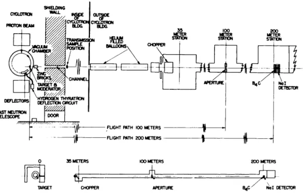
FIG. 1. Geometry of the Columbia University synchrocyclotron slow neutron velocity spectrometer.
T h e lower part of the diagram shows the cyclotron and the 200-meter flight path to scale. T h e upper part enlarges those parts of particular interest.
RECENT VELOCITY SPECTROMETER RESULTS 93
T he duty cycle is 1/100, so t he average intensity is /av = 3 Χ 1 010 neutrons/sec.
I n order to determine t he instantaneous intensity a nd average intensity for t he system we use now, it is necessary to u n d e r s t a nd our present method of operation, so I wil l briefly describe o ur system. Figure 1 shows t he geometry of t he system. T he lower part of the figure is a scale drawing of t he cyclotron, t he shielding, t he
T I M E
2 9 mc
FREQUENCY Of CYCLOTRON OEE VOLTAGE
C2 (TUNED FREQ.) C? GATE
C , (TUNED FREQjj
^ 19 mc
C O I N C I D E N C E - * START PULSE
* 0LOCK ( P U L S E D OSC » FOR BAST C R T S T O R A G E
S Y N C H R O N O U S D R U M B R A C K E T
* * D R U M I N T E R R O G A T E P U L S E S
i L
- 2 0 00 CHANNELS
( . 1 .
2. 4. Β u SEC )] 2m SEC U _ PERIOD FOR C-.R.T I 1 TO DRUM TRANSFER
•llllllllllll
2 0 00 PULSES 7 4 4 μ SEC REP RATE
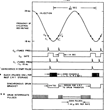
FIG. 2. Timing diagram, t This pulse fires the hydrogen thyratron deflection circuit and turns off the main cyclotron R F oscillator for 2000 μsec.
* T h e iming system clock is driven by the return signal, indicating firing of the deflection pulse circuit. ** Interrogate pulses are for the transfer of the C . R . T . fast (temporary) stored information to the slower magnetic drum storage.
200-meter, flight path, and the detectors. T he upper diagram eliminates most of the 200-meter flight path and gives more details on the cyclotron and the important parts of the flight path.
I n a synchrocyclotron, protons are injected at the center of the machine and accelerated wit h a frequency corresponding to the rest mass of the proton. As the protons are accelerated, the mass increases and the frequency must decrease. Figure 2 shows a timing sequence of the velocity selector system relative to the RF accelerating cycle.
T he upper curve shows the change in RF frequency wit h time.
T he protons are injected at a frequency of about 28 M c and are
0 l"
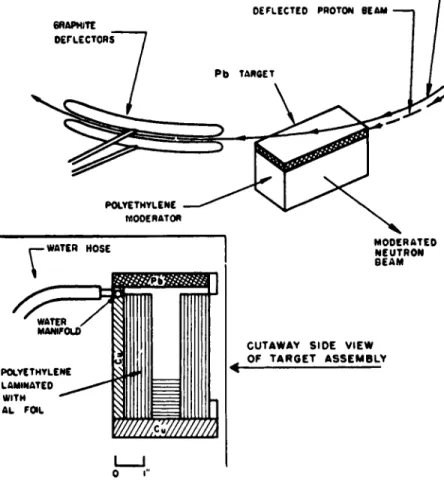
FIG. 3. Schematic diagram of the target assembly and deflectors.
accelerated until the frequency is about 19 M c. We insert a t u n ed circuit into the cyclotron which picks up an RF voltage from the cyclotron and gives a start pulse for the velocity selector system at time C2. T h is tells us that the protons are at the particular radius at which we want to deflect t h e m. T h is signal is sent to a pulse trans- former, which applies a voltage to the deflectors. As shown in Fig. 3, the deflection pulse causes the beam to shift d o w n w a r d;
the pulse has an amplitude of about a h u n d r ed thousand volts and rises in less than a tenth of a microsecond. I n one more revolution the beam hits a lead target about 1 inch below the median plane of the cyclotron. We have tried various targets from beryllium to uranium, and we use lead simply because it leaves the least residual radioactivity. We obtained a few more neutrons from u r a n i u m, b ut the target was so hot that we had to wait 2 weeks after we had stopped operations before anybody could work on the machine, a situation that could not be tolerated.
A moderator is located just below the fast neutron-producing lead targets. T he fast neutrons are practically all evaporation neutrons. T he moderated neutrons travel to our detectors 200 meters away. T he moderator is polyethylene sheets laminated wit h a l u m i n um foil and is water-cooled.
T he factors required to calculate the burst intensity in the Nevis synchrocyclotron are the average beam current, which is 0.5 /xa;
the modulation frequency of 60 cycles giving 60 pulses/sec; and burst width, which is measured by a Cerenkov counter to be 0.025 μ^ο.
W h en we put 400-Mev protons into a target, no matter what the target is, we get about 10 neutrons/proton. T he instantaneous neutron intensity is t h us
r - r , n ,s protons tn neutrons I = 5 X 10-' amp χ 6 Χ 1018 — X 10
amp sec amp sec protons 1 1
60 - 2.5 Χ 1 0- = 2 X 1 0 19 ™ /n se ' e c
T he duty cycle for the Nevis synchrocyclotron is 2.5 X 10~8 X 60 so the average intensity is
/av = 2 Χ ΙΟ19 X 2.5 Χ ΙΟ"8 X 60 = 3 Χ 1013 neutrons/sec. I n 1941 we used two B F3 proportional counters for detectors, each 5 cm in diameter and 20 cm long, at a pressure of 30 cm of H g.
Isotopic B10 was not available, so natural boron, which contains about 2 0% B1 0, was used. Therefore, our original detectors contained 1/30 gm of B1 0. O ur present detector contains 18 kg of B1 0. However, our original detectors were 1 0 0% efficient for detection of the boron disintegration, whil e our present detectors respond to the y-ray emitted in the boron disintegration and the efficiency is only about 1 0 %. Therefore, our detector efficiency has increased by a factor of about 5 Χ 104. T h is is not really a fair comparison, because in 1941 we could not have used a detector wit h as large an area as we use now, b ut it does give you an idea of how m u ch our detector efficiency has increased.
I n addition, we now have a 4000-channel analyzer instead of the single-channel analyzer used originally.
Summarizing the various factors shows an increase of 6 Χ 106 in instantaneous source intensity, 103 in average source intensity, 5 Χ 104 i n detector sensitivity, and 4 Χ 103 in electronic efficiency, for an over- all increase in efficiency of between 2 Χ 1 011 and 1.2 Χ 1 01 5. I t is interesting to note that we are, in effect, using about an " a m p e re of neutrons,'' an enormous current which, w h en combined wit h improved time analyzers and detectors, gives us more t h an 1 011 times the data-taking capacity of 20 years ago. T h is illustrates why some of the future of neutron spectroscopy lies wit h t he machines rather than wit h the choppers.
N ow let us return to the geometry shown in Fig. 1. I n transmission measurements the samples are placed outside the cyclotron shielding.
T h i s shielding is now 6 feet of concrete and 4 feet of steel, and the hole through the concrete and steel is about 3 by 6 inches. O ur beam is defined by three apertures: an aperture t h r o u gh the shielding around the cyclotron, an aperture at 35 meters, and an aperture at 100 meters; there is none near the detector. Actually, the apertures that really define the beam are those at the source and at the
100-meter station.
O ne of the problems which we faced when we went to a 200-meter flight path was that the very low energy neutrons from one burst would overlap the neutrons from the beginning of the second burst.
W e took care of this overlap by putting in a chopper at the 35-meter position. You can see we do not consider choppers completely outdated! T he chopper is not very elaborate; it opens and closes in about a millisecond, not a microsecond. I t is very easy to synchronize to the machine since our machine is synchronized to the 60-cycle
line; we obtain a signal from the chopper as it rotates and move the timing of the deflection pulse in order to deflect the protons at the proper time.
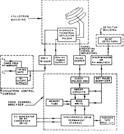
W h en we began operation we encountered several unexpected problems. We had anticipated that we would be able to r un wit h gate widths of 0.05 /xsec, which at a flight path of 200 meters and wit h a source width of 0.025 /*sec gives a resolution of better t h an 0.000375 /xsec/meter. W h en we began to operate wit h 50-nsec gates, everything would operate perfectly for a short while, but then the cyclotron would slip out of phase by about 25 nsec and we would not have proper synchronization. A circuit has been designed which wil l take care of this, and on our next runs we expect to be able to use 50-nsec gates. T he best data we have at the present time were taken on runs using 100-nsec gates. I wil l show you what those data look like. T h e re is information on our circuitry in the Review of Scientific Instruments for May, 1960 which I wil l not repeat here, except to show the block diagram of Fig. 4.
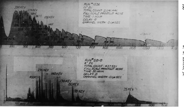
Figure 5 shows the raw data that we obtain from the analog readout of our time analyzer. At the top is the r un n u m b er 1036; a sample containing 1.1 inches of bismuth was in the beam, the total count was 2 millio n in 1 hour, and the channel widths were 0.1 /xsec.
T he y-ray flash occurs in channel 2 1, so that this is the time from which we make all our measurements. I t takes 0.67 /xsec for a y-ray to get from the source to the detector 200 meters away, so our zero time is effectively in channel 15. T he bottom part of Fig. 5 shows the resonance structure from an iron sample 4 inches thick. I have indicated the energy scale as shown. T h is is a transmission curve, wit h a typical interference dip in the cross section at 25 kev for a resonance which is actually at 29 kev. Similarly, as we go up in energy there are interference dips at 70 kev, 80 kev, 130, 140, 290, 400, and so on. You can see that in something lik e iron we are able to separate resonances well above 100 kev. One interesting observation which shows up in the upper part of the slide is a very nice, sharp resonance at 1 Mev. We have helium balloons between the source and detector to reduce the scattering from the nitrogen in air; consequently, we probably have the thickest helium absorber that anyone has ever used to make a transmission measurement. We see the P3 /2 level in helium at 1 M ev which shows up very clearly. R un 1036 shows the sort of resonance structure we obtain in the kev region for bismuth.
T h e re are many more resonances observed in this particular run
cyclotron
b U I L O l N C " ~
TUNED FREQ
RF M A R K E R S
3 0 0 V T R I G G E R
I m SEC G A T E ~T
— RF I I
CUTOFF - J C I R C U I T
IOKV HV
P O W ER
S U P P L Y
I
DETECTOW
£ BUILDING
S C I N T O E T E C T O R S
" 1
"I ι
S I G N A L I N D I C A T I N G F I R I N G OF O E F L E C T O R S
P U L S E S H A P E R
D I S C R I M I N A T O R
OR j
PM A N A L Y S E R
C L O C K ( P U L S E D OSC)
O E T P U L S E Q U A N T I Z E R
L_ 1
• cyclotron control LCONSOLE
2000 CHANNEL ANALYSER
S W E E P C I R C U I T S
M E M O R Y T U B E
Σ Ζ Σ
R E A D W R I T E
A C G E N E R A T O R
ON R F
C O N O E N S E R D R I V E
S Y N C H R O N O U S D R U M P E R M A N E N T
S T O R A G E
P U N C M E O TAPE
IP R I NT υ·.ιΐ
FIG. 4. Block diagram of the electronic system.
One of o ur problems in analyzing t he data is a background which can be seen from t he over-all shape of the envelope of these resonan- ces. W e h ad this background at our 35-meter station a nd h ad hoped that it would disappear when we went o ut to t he 200-meter station;
the 200-meter flight path goes through a tunnel a nd we hoped t he additional shielding would eliminate t he problem. Unfortunately, it did not, so we h ad to employ a very m u ch more elaborate means of than are shown i n this energy region i n any of t he revisions of B N L - 3 2 5. T he large resonances show up very well in t he earlier Van de Graaff data, b ut t he small resonances do not show up at all.
TRA*
FULL ZSC^LZ PRtnTÛJT- *t ' o TIME- / M ? v / ?
CEUM* O '
CHANNEL Ot/sSEC
NE
i l i i i i
FIG. 5 . Raw data from the analog print-out system of the 2000-channel analyzer. In the upper curve a sample of bismuth 1.1 inches thick was in the beam. In the lower curve a sample of iron 4 inches thick was in the beam.
. W. HAVENS, JR.
determining the origin of the background, and we finally traced the background to something wit h which people in the American Nuclear Society should be very familiar. We have, in effect, an iron-moderated neutron source. We have a very intense neutron source at the center of 3000 tons of steel, and consequently we get neutrons coming into the iron, being elastically and inelastically scattered, returning to the moderator, and then being scattered into the flight path. T h e se are neutrons wit h slightly higher energies than those from the initial burst at corresponding times, and because they come right down our flight path they are very difficul t to elimi- nate. Another background which we have is due to capture y-rays which originate in the concrete and in the various portions of the cyclotron shielding behind the source which the detector sees.
W e subtract the background to a first approximation by introducing lead into the beam and varying both sample thickness and filter thickness. We can eliminate the background completely by intro- ducing an auxiliary chopper either 9 meters from the source or 35 meters from the source and synchronizing these choppers wit h the cyclotron. I n view of the results that Rex Fluharty gave on synchronization, I do not think we wil l have any problems if we only have to synchronize the choppers to 10 or 20 /xsec.
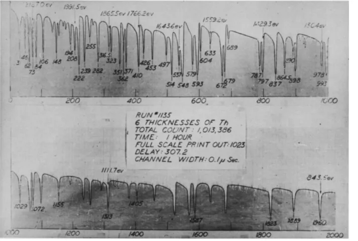
Figures 6 and 7 show some data which may be more interesting from the point of view of reactor physics. We took data on several samples of t h o r i um in these particular runs, wit h good statistics, and we are trying to analyze the data at the present time. T h e se runs (Figs. 6 and 7), wit h two different delays, give an idea of the level structure in thorium. We have been able to do a level-spacing analysis on this. However, we have not as yet determined any resonance parameters. I wil l show later the semianalyzed data from which we worked. R un 1135 (Fig. 6), wit h a 307.2-/xsec delay, took 1 h o ur of operating t i m e; there are a millio n counts in all of these data, and the full scale of the ordinate is 1023 counts. R un 1103 (Fig. 7), wit h a 499.2-/xsec delay, overlaps r un 1135 at the 843.5-ev level.
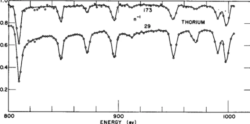
W e have about 300 r u ns of this type, taken in 3 weeks. After we obtained all of these data, we took a week to rest u p, since we ran 24 hours a day for 3 weeks, and t h en began the analysis. Figure 8 shows some old T h data from 800 to 1000 ev which we took at the 35-meter station. T h e se data are shown for comparison wit h the data in the following figures. Figure 9 shows our more recent data
, RUN"/ISS
€ TM/CKNESSES OF Th , TOTAL COUNT : 1,013.366
TIME · / HOUR ; FULL SCALE PRINT OUT/025
DELAY- 307.2
CHANNEL W/DTHO./pS*.
FIG. 6 . Raw data on thorium from the analog print-out system of the 2000-channel analyzer. Delay, 3 0 7 . 2 ftsec.
W. W. HAVENS, JR.
T VELOCITY SPECTROMETER RESULTS
5S
• Ο:-
s 5
1
*>4>4& ·
FIG. 7. Raw data on thorium from the analog print-out system of the 2000-channel analyzer. Delay, 499.2 /usee.
103
taken wit h t he 200-meter flight path in t he region from 800 to 1100 ev. We have data on two sample thicknesses, 1/w = 29 and l/n = 87. T h e se figures illustrate t he resolution we achieve wit h t he 200-meter flight path. I n t he thin sample a small resonance does not show up very well, b ut one does see t he strong resonances i n both
800 900
ENERGY (ev) 1000
FIG. 8. Transmission data on thorium from 800 to 1000 ev taken at the 35-meter detector position.
100 ev lOOOe UOOev
FIG. 9. Transmission data on thorium from 800 to 1100 ev taken at the 200-meter detector station. Upper curve, l/n = 87; lower curve, l/n = 29.
/iOOev /JOOe 1400ev Th
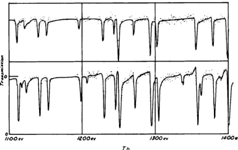
FIG. 10. Transmission data on thorium from 1100 to 1400 ev taken at the 200-meter detector position, f-inch Pb for "open" relative transmission of samples. Upper curve: 2 thicknesses T h -f \ inch Pb, l/n = 87 T h . Lower curve: 6 thicknesses T h , l/n = 29 T h . April, 1961.
I4009V J&OOev /600*v /70Oev
FIG. 11. Transmission data on thorium from 1400 to 1700 ev taken at the 200-meter detector station, f- i n c h Pb for "open." Upper curve: J inch Pb, l/n = 87 T h ; lower curve: l/n = 29 T h . April, 1961.
the thick and the thin samples ; by studying several sample thicknesses we can get some idea of how to analyze these results for the resonance parameters. Since many of you are interested in thorium, I did plot up the thorium results from 800 to 2000 ev; Fig. 10 shows the region from 1100 to 1400 ev, Fig. 11 shows the region from 1400 to 1700,
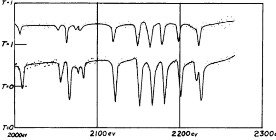
If
2000ev 2\00ev ZZOOev 2300ev
FIG. 12. Transmission data on thorium from 2000 to 2300 ev taken at the 200-meter detector station. Thorium 1147 and 1167. f-inch Pb for
"open." Upper curve: J inch Pb, l/n = 87 T h , Lower curve: l/n = 29 Th. April, 1961.
and Fig. 12 shows the region from 2000 to 2300. T h e se results wil l give you an idea of how good the resolution is. On our next r un we wil l reduce the timing gates by a factor of 2 and have slightly better resolution than shown here.
Figures 13 and 14 show the analysis of level spacings in thorium.
T he integrated distribution of Fig. 13 is shown only to 1300 ev, but it continues linearly. T he other is the distribution of spacings for 63 levels below 1400 ev, compared wit h the Wigner distribution and the random distribution, and I am sure that you are all familiar wit h the fact that the level spacing fits the Wigner distribution.
W e wil l continue to attempt to analyze these data, and I hope eventually that we wil l have a large n u m b er of resonance parameters to give to people who are interested in them. Originally we did not expect to be able to get up to the 100-kev region, b ut it looks lik e we wil l be able to do as well or better than the Van de Graaff machine, even above 100 kev.
60|
50
40
NKE) 30
20
10
Ί — I — I — Γ
D=2I.6EV THORIUM
E —
J I L J I I L
200 400 600 800
EV 1000 1200
FIG. 1 3 . T h e sum from Ε = 0 to Ε of the observed energy levels in T h2 3 2. T h e slope of the curve gives the average level spacing D = 2 1 . 6 ev.
60 70
FIG. 1 4 . T h e distribution of level spacing for T h2 32 for the 6 3 levels below 1 4 0 0 ev.
Discussion
HARVEY: Since your moderator is fairly large, isn't the slowing- down time in the moderator important in the kilovolt energy range, that is, large compared to 0.1 sec ?
HAVENS: N O. T he time required to slow the neutron down is a continuous function of the energy. For 50-nsec gates the dividing point is about 1 kv. For O.l-jusec gates the slowing-down time is equal to the time uncertainty at about 200 volts. T he last collision is the important one.
BROCKHOUSE: IS there any hope of absolutely eliminating that background by phasing the mechanical system ?
HAVENS: Oh, yes. We can put in a chopper in the iron shielding near the cyclotron which wil l open for about 1 /-isec and completely eliminate the background.
MAIENSCHEIN: W i t h the lead target, how long do you have to wait after a 3-week r un to approach the target ?
HAVENS: If we stopped on Saturday morning at 8 A.M., we could get into the machine on M o n d ay morning.