PATH-ADAPTIVE MODE FOR GUIDING SPACE FLIGHT VEHICLES W. E. Minera, D. H. Schmieder

PATH-ADAPTIVE MODE

FOR GUIDING SPACE FLIGHT VEHICLES

W. E. Minera, D. H. Schmieder², and N. J. Braud3 NASA George C. Marshall Space Flight Center, Huntsville, Ala.

ABSTRACT

The need for a more flexible guidance mode than the types now commonly known is established as growing out of require- ments imposed by large staged and clustered space flight vehicles. A new guidance mode is described which meets these requirements and is given the name path-adaptive. The guid- ance functions, which play an important role, are defined in general terms and derived for a simple example. Two methods for the development of guidance functions in practical cases are discussed, and results obtained for an application to a Saturn two-stage vehicle are presented.

INTRODUCTION

With the clustering and staging of rocket propelled vehicles to obtain the capability of injecting multi-ton payloads into lunar and planetary orbits, such as will be done in the Saturn vehicle, there arise certain problems having considerable effect on the design of the guidance system.

First, to obtain a desirable level of reliability with such vehicles, engine-out capability is designed into the propulsion system. This means that a large variation in thrust may be experienced at an unpredictable time on the trajectory. The total energy available to complete the flight is then nearly the same, but the lower thrust lowers the rate at which this energy is available and therefore calls for a differently

Presented at ARS Guidance, Control, and Navigation Conference, Stanford, California, Aug. 7-9, 1961. Revised March 1962.

-^Deputy Chief, Future Projects Branch, Aeroballistics Division.

^Chief, Astronautics Section, Future Projects Branch, Aeroballistics Division.

3Astrospace Technologist, Astronautics Section, Future Projects Branch, Aeroballistics Division.

shaped trajectory.

Second^ the complexity of the vehicle is such that a given liftoff time can be achieved only to an accuracy of several minutes, during which time the launch site and the celestial bodies can change position by a considerable amount.

Also, since the development of such large vehicles is quite expensive, a great variety of missions would be expected to be accomplished with the same basic vehicle design. Besides increasing the costs, a major redesigning between missions would also hurt the reliability of the system.

These factors and others affect the design of the total guidance system, of which the guidance mode is here the subject of interest. The guidance mode should insure the achievement of the missions through the proper operation of the guidance system under these circumstances. The path-adaptive mode is intended to do this, and in such a manner that some prespecified quantity, such as payload, is extremized.

MEED FOR A PATH-ADAPTIVE MODE

The guidance system during flight must in some way obtain information as to the local state (time, thrust acceleration, position, and velocity), make a decision based on this infor- mation as to how the vehicle should be steered, carry out the required maneuvers, and finally terminate the thrust at the proper instant. The plan under which the steering and cutoff decisions are made will be taken here as the definition of guidance mode. This plan then involves a flight theoretical basis for making these decisions in such a way that mission fulfillment will be secured over a certain realm of expected conditions.

For example, under the "delta minimum" mode this is done by always comparing the locally measured values of certain of the state variables with those on a precalculated standard trajectory that is known to cause fulfillment of the mission if followed. The nulling of differences in these variables is then the basis of steering decisions for the vehicle. The realm of expected conditions is assumed to be fairly close to the chosen standard.

Under the "Q-matrix" or "velocity to be gained" mode, the flight is not forced back to a standard trajectory after a disturbance. Instead, an approximation of the vector differ- ence between the locally measured velocity vector and one that if assumed instantaneously would produce mission fulfillment

is computed. Terminating the thrust when the steering maneu- vers based on nulling the vector difference have accomplished that then secures the mission.

Both of the modes just mentioned have been proven successful under the circumstances for which they were developed. When application to the more demanding circumstances imposed by multistage space vehicles with clustered engines is attempted, certain drawbacks are evident. In the case of the delta minimum, the assumption of staying close to a standard trajectory is violated by the altered trajectory necessary for sufficient engine-out performance of the clustered space booster. Satis- factory performance is also a problem in the "velocity to be gained" mode since only indirect control over trajectory shape is held. Also, the various missions to be handled by the large space vehicle do not fit directly into a locally desired velocity vector formulation.

It is probably possible to freeze to some such concept and to engineer extensions that will handle the particular missions as they come up. But the objections still persist that l) knowledge of workability of the modified mode is limited to that one mission; 2) the degree to which the accompanying performance achieves its theoretical optimum is not known; and 3) such modified modes would not lend themselves well to mathe- matical analysis. For reasons such as these, it is considered wiser to abandon the attempt to make such extensions, and rather start afresh with concepts that are independent of mission and vehicle configuration.

Under the path-adaptive mode, the same basic plan is applied to all missions and configurations; to compute continuously the ideal thrust direction program that will satisfy the mission in the most desirable way. "Most desirable" means here that some quantity is to be extremized under given con- straints. That ideal thrust direction should then be adhered to as closely as possible with the hardware available.

These concepts will be elaborated upon in the following paragraphs, and then illustrated by an application to a typical early Saturn study.

OPTIMIZATION CONSIDERATIONS

On contemplating an optimization of the performance associated with the guidance mode, it should be recognized that there are two principal areas over which an optimization may be made.

These are the specific location of the point where mission con- ditions are satisfied and the shape of the thrust direction

function used to acquire that point.

Some feeling for these two areas may be obtained by observing Fig. 1. The mission here could be, for instance, the achieve- ment of an elliptical orbit resulting in certain reentry condi- tions. Then in an assumed two-dimensional flight in the space fixed xy plane, the mission can be represented mathematically by

fj_ (xf, yf, xf, yf, tf ) = 0 i = 1,..., k < 4 [1]

There cannot be more than four independent conditions, for then a fixed point at a fixed absolute time of thrust termination would be implied, which would be very rare as a necessary mission requirement. (In such a case, the guidance problem would be of a very unusual nature, and is not discussed here.) The solution of Eqs. 1 is not unique. For example, any point on curve c of Fig. 1 might represent a solution. Therefore, rather than choose one particular solution as a standard injec- tion point, the mission is left specified in the functional form of Eqs. 1, so that for any given point in phase space

( X Q, y⁰, XQ , jo, t⁰, (F/m)o, (m/m)⁰), guidance may aim at that solution which is the easiest to get to from that point.

This easiest solution already depends on the assumed shaping of the thrust direction history, which is being treated as a second area of optimization. If desired, an arbitrary form of that thrust direction function could be assumed and the corresponding optimization for the best solution of the system of mission Eqs. 1 obtainable with that form made. However, it seems wisest to seek that form which is optimum over all possi- ble functional forms and to use the one function of that family which also provides the optimum solution to the mission Eqs. 1.

This means that among all thrust direction functions that result in curves like a and b in Fig. 1, with end points satis- fying the mission conditions 1 on curve c, the one that mini- mizes some specified quantity is sought. This is the type of problem treated in the calculus of variations, where theory exists providing criteria for singling out the one function that is desired.

SOLUTION FOR STEERING FUNCTION

Consider the vacuum flight of a rocket under constant thrust and mass flow, in an inverse square gravitational field. This physical situation is represented by the system of equations

(F/m)0

(F/m) = [ 2 ]

1 + (m/m)⁰ (t-t⁰) k²

χ

χ

r 3

k2

y = (F/m) cos χ y . [4]

Assume the initial conditions

t0> Jo, io, yo, (F/m)⁰, (m/m)o [5]

to be known and that the mission criteria 1 are to be achieved with a minimum (tf - t⁰) . The X function which does this is determined according to the calculus of variations (1)1 by the satisfaction of

k2

* i = — ^ ( 2 x2- y2) + 3 λ2Χ 7 ] [6]

r ⁵

λ

= —

λ

- χ

) ]

r 5

0

= λχ

λ

simultaneously with Eqs. 2, 3, and 4, and end conditions 1 and 5.

This is a two point boundary value problem. One form of the solution to this problem would be the set of functions x(t), x(t), y(t), x(t), and y(t) that meet the stated requirements, based on no disturbances in the interval (tf - t⁰) . If the solution is made based on an initial point taken later on such a trajectory,the same set of functions x(t), x(t), y(t), x(t), and y(t) would be obtained.

As soon as a disturbance occurs, however, a new set is called for. Thus, the functions X, x, y, x, and y are in turn functions of the initial conditions, and could be written explicitly in

-^Numbers in parentheses indicate References at end of paper.

terms of those initial conditions. Looking especially at the solution for the function x(t), evaluation at t = tQ gives

xo =^xo fro* ^xo> *ο> £⁰> (^F/^m)⁰> ( V m )⁰)

and expresses the solution for the desired thrust direction X0 in terms of the values measured at that initial point. The remaining end conditions that are not given explicitly may be expressed similarly.

The resulting set of equations for the unknown end values in terms of those that are known may be thought of as a second form ofthe solution to the two point boundary value problem.

The most important of these are Eq. 9 and a similar equation for tf. The right hand side of Eq. 9 will be referred to as the steering function while the corresponding expression for tf will be called the cutoff function.

USE OF THE STEERING AND CUTOFF FUNCTIONS

Suppose the steering function given by Eq. 9 were followed exactly during flight. That is, treat each point on the tra- jectory as initial conditions and determine χ0 such that at each point Eq. 9 is satisfied. Then if no further disturbances are encountered, the variable initial conditions would automati- cally change in such a way that again the same curves x(t), x(t), and y(t) would be followed. Under disturbances, however, the adaptive nature of the mode is brought out, for then Eq. 9 automatically initiates the new optimum curves.

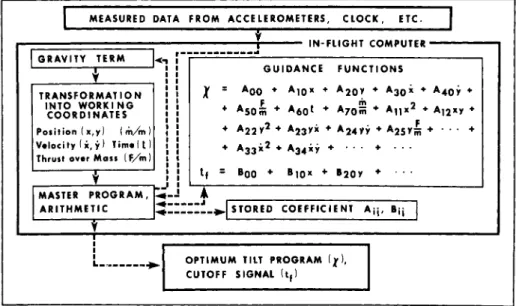
During flight, the steering function value is provided to the system in a manner outlined in Fig. 2 . Here the vehicle is assumed to be at some arbitrary point about which certain measured information is had. This measured data is accepted by the master program and sent through a transformation into the phase space in which Eq. 9 was solved, here termed working coordinates. The master program then calls for the proper steering function and cutoff function forms and the corre- sponding block of stored constant coefficients. The steering function is then evaluated and the resulting value fed out as the ideal thrust direction to be assumed at that arbitrary point.

The control mechanism of the vehicle would then attempt to null the difference between the ideal and the existing thrust directions, until thrust is terminated when tf specified by the cutoff function is reached. The function evaluations are repeated with a frequency depending on the capability of the computer. If this frequency is low, the evaluation of

Χο (*ο> ^xo> ^o* *ο> ^ ο ' (^F/^m)⁰> (^άΑ 0^ο)

may be useful.

The functions used in this manner, including the steering and cutoff functions, will be called collectively the guidance functions. It should be noted that the only change that would occur in the whole setup under a change in mission or configu- ration would be a change in the form and/or stored coefficients of the guidance functions.

The success of an application of the path-adaptive guidance mode is seen to be determined largely by the quality of the guidance functions with which the computer is furnished. This,

in turn, depends on the nature of the function necessary to accomplish the desired results and how well it can be repre- sented for computational purposes. Guidance functions which represent the optimum solution exactly (to measurable accuracy) can be expected to require more computer complexity and weight than simplified approximations to these functions which produce approximate optimums. These tradeoffs should be investigated for the individual applications.

Some methods for deriving guidance functions for the path adaptive mode will now be given.

ANALYTICAL APPROACH TO GUIDANCE FUNCTION REPRESENTATION The second form of the solution to the two point boundary value problem discussed previously (Eqs. 1-8), as represented partly by Eq. 9, may be attempted to be derived analytically.

Conceptually this solution could proceed as in the following simplified example.

Consider the problem of steering a point in (u, v) space from the arbitrary initial conditions

v, ο [10]

to the fulfillment of the mission criteria u^f - U^f = 0

Vf - ¥^f = 0

[11]

[12]

under the equations of motion

û = sin α [13 I

ν = cos α [14^

while minimizing tf - t . Application of the calculus of variations provides the equations defining a

1 1 = 0 [ 1 5 ]

12 = 0 [16]

0 = £1 cos α - i² sin α [17]

having the solution

α - α0 [18]

Substituting this solution into the equations of motion and integrating from t⁰ to the as yet undetermined tf gives

uf - u0 = (tf- t0) s i n aQ [19]

vf - v0 = (tf - tQ) cos aQ [20]

This system is then solved for U f and v^ and substitution made into the mission criteria 11 and 12

uf - uo - (tf - t0) sin a0 [21]

V^f - v^o = (t^f - t^Q) cos a^Q [22]

The simultaneous solution of 21 and 22 provides then the steering function

Uf -uo r ,

aQ = arc tan [23]

Vf - v0

and the cutoff function

t

= t

+V (U

- u

)

+ (Vf - v

)

' [24]

Of course, the derivation does not come so easy for the more realistic problem given by Eqs. 1-6. One approach being investigated is to write the series solution to the initial value problem given by conditions 2-8

,(i)

- Σ τ " -

·

Ο

for u = y, λ.ι , λ² and χ . The coefficients iï

are obtained by successive differentiation^#of Eqs. 2-4, 6-8 and can be written as^functions of X⁰, X⁰, x⁰, XQ , XQ, y⁰, y , t , (F/m^, and (m/m)⁰. Substitution of solution functions 25 into the mission criteria 1 gives a system of equations

[26]

hi (^Xo* *o> *o> ^xo ^ ^xo> ^ο> ?ο> *ο> (^F/m)0> ( * A )0> tf )= 0

i ⁼ 1 , · · · , 4

to be solved for X⁰, &^Q, X⁰, and tf in terms of the other initial conditions. The solution of system 26 would then provide the desired guidance functions.

Various portions of this procedure have been carried out with the use of certain numerical subroutines to replace some of the algebra. The results did not furnish actual guidance functions but did indicate a likelihood that such guidance functions will be possible to derive analytically. Such derivations are desirable both from the standpoint of a check and a guide for the empirical approach to be described next.

EMPIRICAL APPROACH TO GUIDANCE FUNCTION REPRESENTATION In the empirical approach, the two point boundary value problem represented by Eqs. 1-8 is solved numerically with some value assumed for the initial conditions 5 · This is repeated for a large variety of values that lie within a region based on all disturbances the vehicle is designed to withstand. In this way a tabular representation of the guid- ance functions in that region is built up, which may then be approximated by some arbitrary functional form, such as a polynomial. This is a curve fitting problem for functions of several variables, about which no general theory seems to be presently available ( 2 ) . Nevertheless, some fairly good results have been obtained with straight-forward procedures

( 3 ) .

For experimentation with this approach, a two-stage Saturn having a reentry test flight mission was assumed. The mission was to achieve at the depletion cutoff of second stage an altitude of 120 km and a path angle (from the local verticle)

[25]

of 94 degrees. The reentry velocity was to be maximized, with no conditions imposed on the distance down range.

Guidance during first stage was assumed to be already deter- mined by requirements to keep both seven and eight engine flights within limitations on such things as structural loads and swivel angles, since first stage flight took place mostly in the heavy atmosphere. Therefore, the task was to derive a steering function for the vacuum flight second stage whose initial point could be the cutoff point of any such first stage.

No cutoff function was needed because of the depletion cutoff.

The procedure used to build up the table for the steering function was to isolate a family of optimum trajectories origi- nating from the area of first stage cutoff conditions and sat- isfying the reentry mission conditions. The family included trajectories for which variations had been made in the upper stage thrust level, and was comprised of 126 trajectories.

Note that each point on each trajectory of the family can be considered to be another initial condition, and therefore provides another value for the table. Thus, from each trajec- tory of the family points were read every five seconds, pro- viding 12,600 tabulated points of the steering function

Since this mission is independent of time, tQ does not occur in the steering function.

The curve-fitting procedure chosen to represent 27 according to this tabulation was the method of least squares ( 4 ) .

Representation in the resulting polynomial form would be expecially convenient for evaluation by an on-board computer.

The polynomial approximating function used in the least squares procedure may be written in the form

where the summation is taken over a certain set of non-negative integers h, k, p, q, r, s.

The choice of the set of non-negative integers over which the indices range in the summation determines the specific polynomial form being used. For any such choice, it is desired to find the "best'¹ set of coefficients. "Best" can be taken to mean that the differences in the polynomial and tabular value of X are minimized in the sense that the sum of

Xo ^{= X}o (^χο > ^ * O J 7o> (^F/^m) o > (^mA )^Q) [27]

the squares of these differences over all tabulated points is a minimum, i.e.,

Ax(a^hkpqrs)⁼^ [ * b ^ahkpqrs *b *b ΦΙ * [29 \ is a minimum. The index b here ranges over all η of the

tabulated points used, and is the tabulated value of X at the point (x^b, y^b, i^b, y^b, (F/m)^b, (m/m)^b). It is assumed, of course, that the number of tabulated points exceeds the number of coefficients abkpqrs*

A necessary condition for ^ ( a ^ p q p g ) in 2 9 to be a minimum with respect to the a^bkpqrs is that

δ A X ( ah k p q r s)

- o [ 3 0 ]

^ ahkpqrs

for all a^{b k}p q^{r s}. These equations 3 0 are called the normal equations and may be solved simultaneously for the coefficients

ahkpqrs· When written in matrix notation, the solution of equations 3 0 for these coefficients appears as the equation

A = Ν "¹ X [ 3 1 ]

where

Γ . Ί

[ 3 2 ]

A |^(^ahkpqrs)i

N = ( x^hy^kx^py^q ( F / k )^r( i l i A )^e)^;, ( x V i? 7^q( F A )^r( i A )⁸)ⁱ b

X = (xhykxP^(F/m)r(m/m)s)i χ

[ 3 3 ]

[ 3 4 ]

and where i is row index, j column index. In ( ab kp qr se t c . there is a different choice from the set of integers h, k, p, q, r, s for each index i (or j) running from 1 to the number of terms in the polynomial.

A measure of the error due to the approximation by the polynomial thus obtained is given by the expression

v η

[ 3 5 ]

By varying the selection of tabulated points and also the specific polynomial form used in the fitting, one may attempt

to make e as small as possible. The final criteria of good- ness of fit, however, must be a weighing of the number and complexity of terms in the polynomial against the degree of optimization and accuracy of meeting mission conditions achieved by the polynomial.

For fitting the 12,600 point tabulation, various approxi- mating polynomials up through third order were investigated, and it was found that a third order polynomial of eighty-four terms provided the best representation as determined by its error term. Polynomials of this order had error terms of less than .15 degrees. However, work on such high order poly- nomials was not pursued further due to the expected on-board computer storage limitations, especially on early flights of Saturn. Polynomials with from twenty to sixty terms received more emphasis.

A typical example of a polynomial which is a compromise between the number of terms and the accuracy of meeting mission conditions achieved by that polynomial is one which consists of fifty terms in the six variables. Using the 126 trajectories and selecting data in a systematic fashion (1,231 points of the 12,600), the fitting resulted in an error term of .35 degrees. This particular steering function, which consists of first, second and third order terms, was tested by computing trajectories for which the thrust direction was determined by this steering function alone (simulated active guidance). Two cases were checked which originated from second stage initial points lying near the bounds of the region covered by the tabulation. Resulting conditions at second stage cutoff are compared with those occurring on the corresponding optimum trajectories in Fig. 3. The inaccuracies incurred by using this steering function are already quite small, with the

reentry velocity attaining its theoretical maximum value within about .01 percent in both cases.

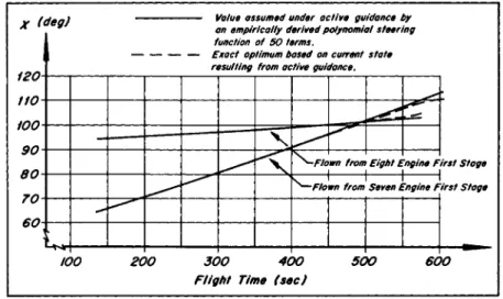
Fig. 4 displays the steering function value time history resulting from simulated active guidance according to the polynomial steering function. The solid curves represent the polynomial value that was flown, and the dashed curves give for comparison the current exact optimum value based always on the existing x, y, x, y, (F/m), and (m/m).

The results are quite good for such a straight-forward pro- cedure, with substantial improvements still to be gained by various techniques. For instance, the selection and distri- bution of tabulated points used, and the adding and dropping of certain terms in the polynomial form seem to have a sizeable

effect on the error term. Also, given a certain polynomial fit, there is the possibility to improve the fit by fitting the residual

to other terms normally of higher order, and then combining the two polynomials. This is being applied to the problem discussed above, and results indicate that the error term can be reduced a great deal by adding only a few residual terms.

There is another tradeoff to be considered, and that is the number of segments of the approximating curve against the degree of polynomial needed to fit each segment. The two extremes would be, an entire stage fit with one function of possibly high degree, and several segments fit linearly. An extension of this would be to carry the 12,600 tabulated

points in the memory of the in-flight computer, and either take the value of the function to be that assumed at the nearest tabulated point, or use a linear interpolation in-flight.

This, of course, would call for an in-flight computer of a different character, but is still a solution to be considered.

SOME ASSOCIATED PROBLEMS

One problem associated with this guidance mode is that of

"mission criteria formulation." In order to know what condi- tions at the end of a propelled phase must be satisfied, the fulfillment of mission conditions must be expressible as certain relationships between those end conditions. This usually involves knowing how the vehicle will move under the influence of gravity due to one or more attracting bodies when the thrust is terminated at a given point, or better, what the point of thrust termination should be in order that the vehicle does move in a certain way afterwards. Given an initial point on a coasting space flight trajectory, that trajectory can be computed and a final point checked against desired mission conditions. By iteration a certain initial condition can be found which does result in the desired mission. But, if this fixed initial condition is given to the vehicle as a propelled phase end condition to meet, it probably will not be able to meet it economically. Thus, what is needed is a general formulation of all end conditions that will result in the desired mission conditions, so that the vehicle can aim at this set of end conditions, always intending to satisfy the one which happens to be optimal for its present situation.

Such a general formulation was represented in systems of Eqs. 1, 11 and 12 in the examples discussed previously. For near Earth missions, such as the reentry example for which numerical results were given, these formulations are usually fairly simple. However, as soon as lunar and planetary missions are brought in, the realm of unsolved classical problems in celestial mechanics is entered.

There are several problems connected with the singling out of the calculus of variations optimum trajectories, both analytically and empirically. The inequalities which can occur in the end conditions and as constraints on the optimum path do not occur in the ordinary statements of applicable theorems. There is also a need to further investigate the requirements at staging discontinuities, and those imposed by further necessary conditions which make up the sufficiency conditions for an optimum solution. Solutions that might exist outside the class considered in the theorems applied should also be considered.

A problem existing especially in the empirical approach to steering function development is the rapid isolation of desired solution trajectories to be fitted. The difficulty here is in working with functions of several variables which are known only through the ability to find the numerical value of the function for given values of the variables.

Also, there is the danger of getting caught in local extremums when the over-all extremum is desired. This problem also appears in performance work.

The problem of empirically fitting the steering function represents an area of mathematics in which very little organized theory has been developed - function approximation for functions of several variables.

Most of these problems are now being attacked at Marshall Space Flight Center and by a group of several university and industrial contractors that meet periodically at the Marshall Space Flight Center.

CONCLUSIONS

A description of the path-adaptive guidance mode and some methods that are now being applied toward the representation of the guidance functions associated with it have been given.

In the light of early results obtained by both an analytical and an empirical approach to the problem, satisfactory solu- tions can be expected to be achieved. Effort should be directed towards the strengthening of the theoretical basis

x, y = space frxed cartesian coordinates, origin at center of earth

r = "\/x2 + y2', distance from center of earth t = time

χ = thrust direction angle, measured clockwise from positive y direction to thrust vector F = thrust magnitude

m — mass of vehicle Λχ, 7\2, i i j i ^ Lagrange multipliers k2 = Gaussian constant

ahkpqrs = coefficients of an approximating polynomial function

Α, Ν, X = matrices defined in text

η = number of tabulated points used in a curve fit e - yΔ^ , an error function

" η

ο = initial point f = terminal point

for the various mathematical procedures involved, improving the degree of approximation achieved in representing the

steering function, developing economical methods of arriving at that function, and examining the effects which will be caused by the various physical parts of the guidance system lagging behind the instantaneous maneuvers assumed in deriving the steering function.

ACKNOWLEDGEMENTS

The authors are indebted to D. 0. Harton and W. L. Perkinson of the General Electric Company group operating digital com- puter facilities at MSFC Computation Division, for the computer programming in this problem.

NOMENCLATURE

b = tabulated point -1 = matrix inverse

A dot over a symbol indicates differentiation with respect to time.

REFERENCES

1 Bliss, G.A#, Lectures on the Calculus of Variations (University of Chicago Press, Chicago, 19U6)

2 Thacker, H.C., Jr., "Numerical properties of functions of more than one independent variable," An. N.Y, A c^# Sc. 86, 677-87U (I960)

3 Schmieder, D.H. and Braud, N.J., "Implementation of the path-adaptive guidance mode in the steering techniques for Saturn - multistage vehicles," Preprint 19U5-6l3 ARS Guidance and Control Conference, Stanford, Calif., Aug. 1961 (the present paper incorporates much of this material)

h Scarborough, J.B., Numerical Mathematical Analysis (Johns Hopkins Press, Baltimore, T O T

E l l i p s e nc " R e p r e s e n t i n g M i s s i o n

Fig. 1 Choice of path and injection point

j M E A S U R E D DATA F R O M AC CE L Ε R O M E T E R S , C L O C K , E T C

' I

G R A V I T Y T E R M 1

IN-FLIGHT COMPUTER-

T R A N S F O R M A T I O N I N T O W O R K I N G

C O O R D I N A T E S Position ( x,y) ( m/m ) Velocity (x,y) TIMET t ) Thrust over Mass (F/m)

Τ

MASTER PROGRAM, ARITHMETIC

GUIDANCE FUNCTIONS

Ϊ = AQO • ^A1 0^x * A2OY * ^A3 o^x * ^A4OY *

* Α5 θ £ + A6 0T • A70ïS *^Απχ 2 * AI2XY *

• 2 2Α γ 2 + 2 3A v x + A24YY + A2 5 y m • · · · •

* 3 3Α χ 2 + Α3 4χν + . . . + . . . TF ^{= BQO +} B l Ox + B²O Y • ·

Λ S T O R E D C O E F F I C I E N T A :

O P T I M U M T I L T P R O G R A M {χ), C U T O F F S I G N A L ( tf)

Fig. 2 In-flight use of guidance functions

Quantity *Based On a First Stage of:

Initial Value, Ideal Traj.

Terminal Value, Ideal Traj.

Terminal Deviation Under Guidance t

(sec)

Eight Engines Seven Engines

146.9 166.2

611.2 630.5

0.0 0.0 X

(deg) Eight Engines Seven Engines

94.6 67.3

103.5

115.8 —

Velocity (m/sec)

Eight Engines Seven Engines

2,977.3 2,931.9

8,855.1 8,965.0

0.7 0.4 Path Angle

(deg)

Eight Engines Seven Engines

55.7 66,0

94.0 94.0

0.02 -0.01 Altitude

(km)

Eight Engines Seven Engines

92.4 75.5

120.0 120.0

0.1 -0.1

*Both cases fly same first stage tilt program designed to meet control and hardware requirements

Figo 3 Mission miss resulting from the simulated use of an empirically derived polynomial steering function having ï>0 terms. Application is to the second stage of a re-entry test flight

X (deg) Value assumed under active guidance by an empirically derived polynomial steering function of 50 terms.

Exact optimum based on current state resulting from active guidance.

100 200 300 400 Flight Time (sec)

500 600

Fig. U Comparison between the steering function values that were flown (simulated flight) and the current exact

optimum steering angle (*)0