GEOGRAPHICAL ECONOMICS

(1)

GEOGRAPHICAL ECONOMICS

(2)

(3)

(4)

ELTE Faculty of Social Sciences, Department of Economics

Geographical Economics

week 8

KRUGMAN (1991) MODEL: DYNAMICS AND SIMULATION Author: Gábor Békés, Sarolta Rózsás

Supervised by Gábor Békés

June 2011

(5)

week 8 Gábor Békés

Krugman model 2:

dynamics Equilibrium and simulations Equilibrium Results and history

Outline

1 Krugman model 2: dynamics Equilibrium and simulations Equilibrium

Results and history

(6)

Krugman model 2:

Equilibrium

Krugman (1991) model - continuation Dynamics, equilibrium

BGM Chapter 4.2-4.4 BGM Chapter 4.5 in part

Krugman's slogan: geographical economics model =

1 Dixit-Stiglitz core

2 + icebergs

3 + evolution

4 + a computer

(7)

Krugman model 2:

Equilibrium

Very dicult, non-linear model

How can we calculate an equilibrium for a given distribution ofλ?

1 Determining the exogenous parameters

2 and using a computer for simulations. . .

(8)

Krugman model 2:

The model

The model, if φ₁ =φ₂=0.5

Y₁ =λ₁W₁δ+₀.5(₁−δ);Y₂=λ₂W₂δ+₀.5(₁−δ) ₍₁₎ I₁= (λ₁W₁¹⁻ê+λ₂W₂¹⁻êT¹⁻ê)¹^/(¹⁻ê); (2) I₂= (λ₁T¹^−eW₁¹^−e+λ₂W₂¹^−e)¹^/(¹^−e) (3)

W₁ = [Y₁I₁ê⁻¹+Y₂T¹⁻êI₂ê⁻¹]¹^/e; (4) W₂ = [_Y₁_T¹⁻ê_I₁ê⁻¹+_Y₂_I₂ê⁻¹]¹^/e ₍₅₎

w₁ =_W₁_I₁^−δ;w₂ =_W₂_I₂^−δ ₍₆₎

(9)

Krugman model 2:

Parameters

How should we choose the values of parameters for the simulation?

Empirical observations Round numbers Usefulness. . . δ=₀.4

L=1

λ₁+_λ₂=₁ φ₁=φ₂=₀.5 e=5

ρ=₁−_1/5=₀.8 1/(₁−e) =−0.25 T =₁.7

T¹⁻^e=₀,12

(10)

Krugman model 2:

The model

After normalization and simplications

Y₁=0.4λ₁W₁+0.3;Y₂ =0.4λ₂W₂δ+0.3 (7) I₁= (λ₁W₁⁻⁴+₀,12λ₂W₂⁻⁴)⁻⁰^.²⁵; (8) I₂= (0,12λ₁W₁⁻⁴+λ₂W₂⁻⁴)⁻⁰^,²⁵ (9)

W₁ = [_Y₁_I₁⁴+₀,12Y₂I⁴)⁰^,²⁵; (10) W₂ = [0,12Y₁I₁⁴+Y₂I₂⁴]⁰^,²⁵ (11)

w₁=W₁I₁⁻⁰^,⁴;w₂ =W₂I₂⁻⁰^,⁴ (12)

(11)

Krugman model 2:

Procedure

Sequential iteration

Denition: W₁,5:=the value of W₁after the fth iteration (_it)

Guess an initial solution for the wage rate in the two regions (W₁,0=_W₂_,₀=1), where 0 indicates the number of iterations

Calculate the income levels (Y₁,0Y₂,0) and price indices (I₁,0

I₂,0)

Substitute and determine a new possible solution for the wage rates (W₁,1,W₂,1)

Repeat these steps until a solution is found: when W barely changes

(W_r,_it−W_r,_it₋₁)/W_r,_it₋₁<σ, for each r =1,2 σ:=₀.0001

(12)

Krugman model 2:

Relative real wage

Real wages are the incentive to move

When we get the short-run equilibrium setting (I,Y,W ) ⇒ we can calculate the ratio w₁/w₂

Figure on real wages

Simulations - x a given value ofλ₁and seek the equilibrium values of variables to this

Execute this program several times, varyingλ₁between zero and one

Plotting the relative real wage in region 1 against the value of λ₁

Equilibrium, if

w₁/w₂=_{1 and 0}<_λ₁<_{1 or} complete agglomeration (λ₁=_{1 or 0)}

(13)

Krugman model 2:

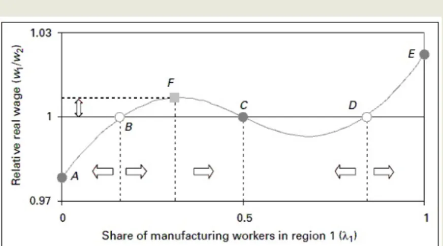
Figure on the relative real wage

(14)

Krugman model 2:

Figure on the relative real wage (2)

There are three types of equilibrium

A,E - complete agglomeration of manufacturing production C - spreading of manufacturing production over the two regions

B,D - manufacturing production is partially agglomerated Total of ve long-run equilibria

3 equilibria `nding' them analytically (guessing) (A,E,C) 2 equilibria nding them with simulations (B,D)

(15)

Krugman model 2:

Stability

Stability (on the basis of w₁/w₂)

Suppose, e.g., that we are in point F ; w₁ is greater than w₂, therefore it is worth moving to R1 (λ₁increases), and get to point C.

It is valid for any arbitrary point between points B and C When the economy is located somewhere between point B and D, it reaches the spreading equilibrium sooner or later.

This point is the basin of attraction for the spreading equilibrium.

Similar reasonings hold for the segments between points A and B and between points D and E. They are called the basin of attraction for the agglomeration equilibrium.

(16)

Krugman model 2:

Instability of equilibria

There are two points (B and D), that are equilibria, but unstable.

If the economy `falls' exactly in these points, it will stay there (real wages are equal)

Any arbitrarily small perturbation of this equilibrium will set in motion a process of adjustment. . .

(17)

Krugman model 2:

Figure on transport costs

(18)

Krugman model 2:

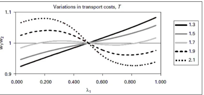
The eect of transport costs

Recall: transport (transaction) costs are the `heart' of the model, the most important exogenous factor

Repeating the previous procedure for T ={1.3,1.5,1.7,1.9,2.1}

If transport costs are large (T =₁.9 or T =₂.1), the spreading equilibrium is the globally (unique) stable equilibrium

When the two regions are too far away from each other, it is not worth producing in either of them and shipping to the other.

If transport costs are smaller (T =1.3 or T =1.5), the agglomerating equilibria are stable

If the two regions are very close to each other, the one that has a production cost-advantage (lower wage), will be the

`winner' (complete agglomeration).

The spreading equilibrium exists but unstable!

T =₁.7 - there exist more equilibria. How special is this settings?

Not so frequent

But it always exists (for each parameter setting can be assigned a particular T )

(19)

Krugman model 2:

Figure on transport costs

(20)

Krugman model 2:

The eect of changes in transport costs

Put the equilibrium distribution of mobile workforce λon the vertical axis and transport costs T along the horizontal axis S sustain point - until which complete agglomerations are equilibria

B break point - from which the spreading is equilibrium The segment between points B and S may be arbitrarily small or even a point.

>The tomahawk diagram

(21)

Krugman model 2:

The `tomahawk' diagram (a)

(22)

Krugman model 2:

Agglomeration equilibrium (Reminder)

All manufacturing workers are located in one of the regions.

Agglomeration in region 1 (λ₁=₁,λ₂ =₀₎ W₁ =1

Then I₁=₁,I₂=_T

and Y₁= (1+δ)/2,Y₂= (1−δ)/2 W₁ =₁,w₁ =₁

W₂ =[(₁+δ)_/2]_T¹^−e+ (₁−δ)_/2]_Tê−¹ ¹^/e w₂ê = [(₁+δ)_/2]_T¹⁻ê⁻êδ+ (₁−δ)_/2]_Tê⁻¹⁻êδ

If T is nor too large (but T >_{1), w}₂<1, i.e. nobody wants to move

(23)

Krugman model 2:

Sustain point (S)

What does the assumption `T is not too large' mean? We can determine a sustain point (S):

w₂ê =f(T) = [(1+δ)/2]T¹⁻ê⁻êδ+ (1−δ)/2]Tê⁻¹⁻êδ=1

⇒_S(_T)'₁.81

(24)

Krugman model 2:

Sustain point (S)

What does the assumption `T is not too large' mean? We can determine a sustain point (S):

w₂^e =_f(_T) = [(₁+δ)_/2]_T¹^−e−eδ+ (₁−δ)_/2]_T^e−¹^−eδ=₁

⇒T '1.81

As transport costs increase, however, the rst term in the above equation becomes arbitrarily small, while the second term becomes arbitrarily large if

1−e−eδ>0⇒1−e>eδ⇒(1−e)/e>δ⇒ρ>δ ρ>δ= no-black-hole condition if this condition is not fullled the forces working toward agglomeration would always prevail (independently from transport costs), and the economy would tend to collapse into a point.

(25)

Krugman model 2:

Symmetry break point (B)

Break point (B) - from which the spreading equilibrium is stable

Recall: Ha W₁=_W₂=₁

Then I₁=_I₂= (₀.5)¹^/(¹^−e)(₁+_T¹^−e)¹^/(¹^−e) and Y₁=_Y₂=₀.5

W₁ =₁=_W₂,és w₁ =_w₂ : this is an equilibrium We can show, that the condition necessary to break the spreading equilibrium, i.e., dw/dλ>0

g(T):= ¹−T¹^−e

1+_T¹^−e + [1−^δ(₁+ρ)

δ²+ρ ]<1 (13) The rst term on the right-hand side is Z ∈(₀,1) _{and is} monotonically increasing in transport costs T, while the second term is a constant fraction strictly in between zero and one (if the no-black-hole condition is fullled). See the gure above!

Now B(T)'1.63

(26)

Krugman model 2:

Krugman-Fujita-Venables (1999) Theorem

Theorem

Suppose the no-black-hole condition (ρ>δ) holds in a symmetric two-region setting of the Krugman model, then (i) complete agglomeration of manufacturing activity is not sustainable for suciently large transport costs T, and (ii) spreading is a stable equilibrium for suciently large transport costs T.

(27)

Krugman model 2:

History matters! (1)

An important implication of the model

Case A: Transport costs are large, e.g., T =₂.5, and the spreading equilibrium is stable

Suppose that transport costs start to fall, T =₁.7 - as B(T)=1.63, the spreading equilibrium remains stable Case B: Transport costs are large, e.g., T =₁.3, then agglomeration equilibrium is established in one of the two regions

Suppose that transport costs start to rise, T =_{1.7 - as} S(T)=1.81, nothing happens. Agglomeration of manufacturing activity remains a stable equilibrium That is, in the case of T =₁.7, the outcome equilibrium depends on history.

= "Evolution"

(28)

Krugman model 2:

History matters! (2)

Go back to the `tomahawk' diagram. Suppose that transport costs are large and we begin to reduce them (e.g.

technological progress).

(29)

Krugman model 2:

History matters! (2a)

Go back to the `tomahawk' diagram. Suppose that transport costs are large and we begin to reduce them (e.g.

technological progress).

Until a particular point there is symmetry, then the economy sharply renders to agglomeration

Recall: Letη be the speed of adjustment and w is the weighted average of the real wages (w =λ₁w₁+λ₂w₂)_. Then the motion of manufacturing labor can be described by this simple dynamic system: ^d_λ^λ₁¹ =η(w₁−w)

Which of the regions?

The one to which the rst migrant decides to move or the outcome is solely the result of a historical accident Non-linear relationship!

Due to a small step the economy suddenly reaches one of the agglomeration equilibria

T falls until a particular point nothing happens T falls further sudden powerful change