PhD Thesis
Further development and novel applications of the Robust Fixed Point Transformation-based adaptive
control
Krisztián Kósi
Supervisor:
Prof. Dr. habil József Kázmér Tar DSc.
Doctoral School of Applied Informatics and Applied Mathematics
Budapest, 20th Aug. 2015
Members of the Defense Committee:
Day of the defense:
1 Introduction 1
1.1 Outline of the Main Problems in my Research . . . 2
2 Strict Scientific antecedents of the Thesis 4 2.1 Brief Introduction for the RFPT-based Method . . . 4
2.2 Early Parameter Tuning in the RFPT-based Method . . . 6
2.3 Fractional Derivatives . . . 7
2.4 Order Reduction Techniques . . . 8
3 Investigation of the Robust Fixed Point Transformation based controller outside of the region of convergence 10 3.1 Investigation of Chaos formation . . . 10
3.1.1 Simulations for the Chaotic Regime of a 2 DOF System . . . 11
3.1.2 Chaos Reduction by Smoothing . . . 13
3.1.3 A 3 DOF System . . . 17
3.1.4 Simulation Results and Chaos Patterns . . . 18
3.2 Investigating Asymmetries in Chemical Systems . . . 23
3.2.1 Challenges in Controlling Chemical Systems . . . 23
3.2.2 The Particular Paradigms Under Consideration . . . 24
3.2.3 RFPT-based Adaptive Control of the Brusselator Model . . . 24
3.2.4 Input Coupling in the Control of the Brusselator Model . . . 27
3.2.5 Application of the RPFPT-based Technique for this Chemical System . . . 31
3.2.6 Simulation Results for the Input Coupling Approach . . . 32
3.2.7 The RFPT Method for the Brusselator Model using Fractional Order Derivatives . 33 3.2.8 Simulation Results for the Use of the Fractional Derivatives . . . 35
3.3 Improvement of Extension from SISO to MIMO in RFPT-based Systems . . . 42
3.3.1 Systematic Extension of the RFPT-based Method from SISO to MIMO Systems . 42 3.3.2 More simple extension from SISO to MIMO systems in the RFPT-based adaptive control . . . 43
4 Improvement of the stability of the RFPT-based adaptive control 45 4.1 Improved parameter tuning: “Precursor Oscillations” . . . 45
4.1.1 The RFPT-based MRAC Controller for a 2 DoF TORA System . . . 47
4.1.1.1 The Tuned RFPT-based MRAC Controller . . . 48
4.1.1.2 Simulations for Big NegativeKcandBc= 1 . . . 48
4.1.1.3 Simulations for Big PositiveKcandBc=−1 . . . 50
4.2 The Global Behavior of the Bounded RFPT . . . 51
4.3 Simulations for a 1 DoF Nonlinear System . . . 55
5 Modifications for the original RFPT based control 58 5.1 Tuning of the applied sigmoid function . . . 58
5.1.1 The Sigmoid Function . . . 58
5.1.2 Fine Tuning Results . . . 58
5.1.3 Simulation for TORA system using Fine Tuning method . . . 65
5.2 Combination with the Luenberger observer . . . 70
6 Novel applications of the fixed point transformation based adaptive controllers 79 6.1 Applications in control of the small airplane motion and airplane components . . . 79
6.1.1 Adaptive control of aeroelastic wing component . . . 79
6.1.1.1 Simulation results . . . 81
6.1.2 Control for a small airplane . . . 85
6.1.2.1 The Linearized Small Airplane Model . . . 85
6.1.2.2 Simulation Results . . . 87
6.1.2.3 The Effects of Even Parameter Errors and External Perturbations . . . . 87
6.1.2.4 The Effects of Uneven Modeling Errors and External Perturbations . . . 90
6.2 Novel application for order reduction in the control of a WMR . . . 92
6.2.1 The Kinematic Model . . . 92
6.2.2 Kinematically Formulated Desired Trajectory Tracking for the Given Kinematic Constraints . . . 92
6.2.3 The Dynamic Model of the Cart . . . 93
6.2.4 The Model of The DC Motors . . . 94
6.2.5 The RFPT-Based Design for Order Reduced Adaptive Controller . . . 94
6.2.6 Simulation Results . . . 95
6.3 Adaptive control for 4th order dynamic systems. . . 99
6.3.1 Dynamically coupled SISO systems . . . 99
6.3.1.1 The Model of the4thOrder System . . . 99
6.3.1.2 Simulation Problems in the Numerical Computation of Higher Order Derivatives . . . 100
6.3.1.3 Polynomial Estimator for Higher Order Derivatives . . . 101
6.3.1.4 The RFPT-based Adaptive Control of the4thOrder System . . . 103
6.3.2 Dynamically coupled MIMO systems . . . 105
6.3.2.1 The Dynamic Model of the System to be Controlled . . . 105
6.3.2.2 The Controller Based on the Exact Model . . . 105
6.3.2.3 The Adaptive Controller based on the Approximate Model . . . 106
6.3.2.4 Simulation Results . . . 107
6.4 Application in vehicle control . . . 113
6.4.1 Control of caster-supported carts with two driving wheels . . . 113
6.4.1.1 Simulation Results . . . 117
6.4.2 Nonlinear Order Reduction based on an Adaptive Controller Using Approximate Dynamical Model . . . 119
6.4.3 The Model of the Permanent Magnet DC Motor and the Unified Model . . . 119
6.4.4 Possible Trajectory Tracking Prescriptions Allowed by the Kinematic Constraints 120 6.4.5 Simulation Results . . . 124
6.4.5.0.1 Exact model parameters . . . 124
6.4.5.0.2 Approximate model parameters . . . 124 6.5 Further research plans: Cognitive Control (CoCo) . . . 128
7 Theses 130
8 References 134
8.1 Own publications strictly related to the Thesis . . . 134 8.2 Other own publications . . . 135
I would like to thank all of the support to my supervisor Prof. József Kázmér Tar.
I also would like to express my thank for the professional support of Prof. I.J. Rudas, and Prof. János F. Bitó.
I also would like to acknowledge for the professional and administrative support to Prof. László Horváth and Prof. Aurél Galántai of the Doctoral School of Applied Informatics and Applied Mathematics.
I am very thankful to Prof. Márta Takács for guiding me in the realm of the Fuzzy systems and soft computing.
I am also very thankful for my Mother and Father for they permanent incentives.
INTRODUCTION
Iterative techniques as numerical methods are widely used for finding the solutions to typically non- linear problems for which normally no closed-form analytical solutions exist. The classical Newton- Raphson algorithm that was developed in the17thcentury [1] obtained wide attention even in our days (e.g. [2, 3, 4]). It is aroot finding algorithmin which the original task is transformed to afixed point problemthat is solved via iteration. The convergence properties of such iterative sequences were sys- tematically studied by Stefan Banach in 1922 in hisFixed Point Theorem[5]. Techniques for speeding up the convergence of iterative sequences were also introduced in the20thcentury (e.g. [6, 7]).
Robotics is a typical subject area in which strongly nonlinear systems have to be controlled. The method ofIterative Learning Control (ILC)applied in robotics was at first announced in English by Ari- moto in 1984 [8]. It also obtained various applicationswhenever the task of the robot is to repeatedly reproduce a typical motion(e.g. [9], [10], [11]). By the application of the concept ofmotor primitives similar approach was recently applied by Deniša et al. in [12].
In a wider context in robotics i.e. when the robot has to precisely track anominal motionthat is not periodic the classical adaptive control approaches normally use Lyapunov’s2ndor “direct” method that originally was developed for the investigation of the stability of motion of nonlinear systems in the last decade of the19th century [13]. In the sixties of the past century his work was translated to English [14] and became the mathematical basis in nonlinear adaptive control design. Its great advantage is that even in the lack of the existence of closed analytical solutions of the equations of motion various stability definitions can be proved for the controlled motion without knowing its other details.The classic examples as theAdaptive Inverse Dynamics Controller (AIDC), theAdaptive Slotine-Li Controller (ASLC) [15, 16] as well as theModel Reference Adaptive Controllers (MRAC)(e.g. [17, 18, 19]) were designed by the us of various Lyapunov functions.
In spite of its great advantages this design technology has some drawbacks. At first it is a “compli- cated” method often burdened by mathematical difficulties. It is easy to see that these mathematical difficulties mainly originate from affording certain “unnecessary luxuries” as follows: the method of- ten guaranteesglobal stabilitythat is practically too much: in the practice both the unknown external disturbances and the model parameter uncertainties areboundedtherefore it is not compulsory to guarantee stability for arbitrarily big model errors, disturbances, and initial states e.g. [20]; the majority of the so designed controllers does not sharply distinguish between the physical role of thekinematic and thedynamicdetails: sometimes force terms are directly fed back without using the dynamic model of the system that results in complicated proofs. Furthermore, the method tries to satisfysatisfactory conditionsinsteadnecessaryones that practically also is “too much”; the solutions normally contain a great number of more or less arbitrary parameters; their optimal setting may need the application of
complicated evolutionary technologies (e.g. [21, 22]).
In order to avoid the mathematical complications related to the Lyapunov function-based design techniques, as alternative approach, iterative solutions were introduced in adaptive control of robots and other nonlinear systems that have to follow in general non-periodic nominal motion with the sig- nificant main characteristic features as follows: a) by applying “sterile distinction” between the role of kinematicsanddynamicspurely kinematic formulation of the desired tracking error damping was pre- scribed; b) the necessary control forces (or other control signals in the case of phenomenologically different physical systems) were calculated on the basis of an available approximate and even incom- plete dynamic model; c) by observing the actual response of the controlled system and comparing this response with the model-based expectation the input of the approximate model was iteratively deformed to better approximate the kinematically prescribed“desired response”; d) the iteration was generated by a fixed point transformation; e) the need for global stability was generally given up.
In [23] and certain related publications transformations based on simple geometric interpretation were introduced and their applicability for various physical systems were clarified. In 2009 one of these transformations, the“Robust Fixed Point Transformations (RFPT)”were found to be especially efficient [24]. The method contained only a single kinematic and only three adaptive control parameters and found numerous potential applications e.g. adaptive optimal dynamic control for nonholonomic sys- tems [25], quasi-stationary control approach in adaptive emission control of freeway traffic [26], etc.
1.1 Outline of the Main Problems in my Research
In my research, the goal was to improve the stability and usability of the nonlinear adaptive controllers. I chose the Robust Fixed Point Transformation (RFPT)-based iterative solutions instead of the Lyapunov function-based technique for the basis of the research, which was developed by J. K. Tar in 2009 [24].
In my thesis new contributions related to this new technique are considered. Accordingly, this research had the logical structure as follows:
1. The original investigations related to the method announced in [24] were restricted to the opera- tion of the controller in the convergent regime. The methods that were elaborated for tuning one of the adaptive control parameters in [27, 28] essentially were restricted to and effective within the convergent regime that was determined by thelocal properties of the fixed point transfor- mation and the response function near the useful fixed point. In [29] the appearance of small fluctuations of the control signal was observed and reduced in the case of a SISO system. No systematic investigations were done to reveal what happens if the controller leaves this regime for MIMO systems. These investigations were initiated by me at first for a 2DOF system [A. 1], later for a 3DOF one [A. 2], and for a chemical system using Brusselator model [A. 3], [A. 4], [A. 5].
It turned out that these controllers produce bounded chaotic motion outside of the region of con- vergence. By the use of affine approximation of the response functions I systematically studied this motion. It turned out that the main features of this motion depend on the global properties of the function that realizes the fixed point transformation and also depends on the properties of the system’s response function. I also invented a novel method to extend SISO Robust Fixed Point Transformation method for MIMO systems.
2. Using the results of the investigation of chaos formation, I realized that at appropriate adaptive control parameter setting continuous increase of the tuned parameter at first produces mono- tonic convergence with increasing convergence speed, then, before skipping into the chaotic regime, it yields non-monotonic convergence with decreasing speed of convergence. I referred to this phenomenon as “precursor oscillations”. I introduced a novel method to stabilize the control system by using a model-independent observer for the precursor oscillations in the parameter tuning process [A. 6], [A. 7].
3. To improve the usability of the original Robust Fixed Point Transformation method, I suggested a truncated linear sigmoid function to replace its original main component with a practically simpler realization. I also introduced a tuning method for it [A. 8],[A. 9].
4. I combined the RFPT-based technique with the application of the classical Luenberger observer for cases in which the system’s state cannot fully and directly measured [A. 10].
STRICT SCIENTIFIC ANTECEDENTS OF THE THESIS
2.1 Brief Introduction for the RFPT-based Method
The great majority of control literature applies Lyapunov’s 2nd method ([13], [14]) for designingglobally stable adaptivecontrollers for both linear and nonlinear systems when the available system models are imprecise and the presence of unknown external perturbations is expected. While the design of model based predictive controllerson the basis of Lyapunov’s technique is relatively easy, the adaptive ones can be designed in a complicated manner is which numerous control parameters can arbitrarily set and the subtle details of trajectory tracking are not well revealed. Both “simple adaptive” as well as “Model Reference Adaptive Controllers (MRAC)” can be designed in this manner (examples from the early nineties of the past century to our days are [15], [16], [17], [30], [18], [31], [19], [32], [33], [34]).
Regarding the details of trajectory tracking as well as finding the appropriate Lyapunov function itself evolutionary methods can be applied, too [21].
Though Lyapunov’s method has the great virtue that it normally guaranteesglobal stability, it also has certain drawbacks as follows:
• The primary intent of the designer of the controller may be to impose precise restrictions on the tracking error relaxation as the controller “learns” or tunes itself. However, these details are not in the focus of the design and they can be revealed only by numerical computations.
• Normally the Lyapunov function may containample number of arbitrary adaptive control param- eters(mainly among the matrix elements of positive definite symmetric matrices). The global stability can be guaranteed for various settings that have significant effects on the details of the controlled motion. For determining the practically satisfactory setting some optimization can be done even by the use of the means ofevolutionary computations(e.g., [35], [22]) that normally may mean high computational burden.
• Though it is easy to understand the mathematical essence of Lyapunov’s method, its particular applications require very good skills on behalf of the designer.
• The method is built up onrather satisfactory than necessary conditions, consequently it normally requires“too much”, i.e., it works with more than necessary stipulations.
• These stipulations mainly originate fromformal considerationsand do not allow the method to become “versatile enough”. For instance, it was recently shown that slight modification of the parameter tuning rules of the “classic”Adaptive Inverse Dynamics Controllerand the Slotine-Li
Adaptive Controller, due to which the tuning rules were not deduced from a Lyapunov function it became possible to combine a modern adaptive technique with the classic parameter learning methods [36], [37].
To evade the above difficulties, an alternative adaptive design method, theRobust Fixed Point Trans- formations(RFPT)-based design was introduced [24]. Realizing that though global stability (if it is guar- anteed) is an advantage but from practical point of view it is “too much” (the modern robust controllers are designed for bounded/limited uncertainties e.g. [20]), insisting on it is not necessary if the prices are increased computational costs and further complications in the design, alternative solutions were initiated in [23] and the related publications. This method applies a particular iterative learning control in which the iterative sequence is obtained by the use of a contractive map in a Banach Space and it converges on the basis of Banach’sFixed Point Theorem[5]. Furthermore it places into the focus the realization of a prescribed trajectory tracking error relaxation. In its simplest form it only needs 3 adaptive parameters that can be fixed for many applications. It can guarantee only a bounded basin of convergence that may be left by the system. If it is necessary for maintaining the convergence, one of its parameters can be adaptively tuned by various manners (e.g., [27], [28]). With the introduction of these tuning rules only a few new parameters are introduced that have well identified roles. This design has the advantage that it does not need any precise initial model of the system under control.
It can do with a very approximate model: without trying to “amend” this model it adaptively deforms its input via observing the behavior of the controlled system. It can well compensate the simultane- ous effects of modeling errors and unknown, directly not observable external disturbances. (Since no model improvement happens, this control permanently needs fresh observations and cannot promise asymptotic stability.)
The most successful version was based on the application of the “Robust Fixed Point Transforma- tions (RFPT)” [24] for the applicability of which it was assumed that the controlledsystem’s response (e.g. acceleration in Classical Mechanics) to the primary controlling physical agent (e.g. torque or force components) is directlyobservable. (This condition normally is satisfied e.g. in robotics). In this case, by the use of anapproximate system modelthe necessary force or other control action for a purely kinematically calculated “desired response”rDescan be estimated and exerted on the controlled sys- tem that produces the observed responser. In this manner a “response function”f(rDes, . . .)can be introduced that is not known analytically but can be identified as pairs of known input and output val- ues. The symbol “. . .” stands for the other arguments off that partly describe the actual state of the system and the variables of the environmental interactions.
The essence of RFPT is to generate acontractive mapGby the use of which instead of directly applyingrDesaniterative control sequencedefined asrn+1 =G(
rn, f(rn), rn+1Des)
is generated in alinear, normed, complete metric space(Banach space). Due to the completeness of the space this sequence has to converge to somer⋆that is afixed pointofG:r⋆=G(
r⋆, f(r⋆), rn+1Des)
. IfGis so constructed that f(r⋆) =rn+1Des this sequence yields the solution of the control task. In [24] the following function was introduced forSingle Input - Single Output (SISO)systems:
G(
rn, f(rn), rn+1Des) :=
(rn+Kc)(
1 +Bcσ( Ac[
f(rn)−rn+1Des]))
−Kc (2.1)
with a monotone increasing smooth sigmoid functionσ(x)∈(−1,+1)also satisfying the requirements σ(0) = 0and dσ(x)dx |x=0 = 1,Bc =±1, and Kc andAc are adaptive control parameters. Since f and thereforeGare related to certain derivatives of the state variable of the controlled system normally rDesvaries slowly and its other variables denoted by “. . .” can be regarded as parameters. The original idea in [24] concentrated only on the condition of the derivative ofGinr⋆in (2.2)
dG(rn,f(rn),rn+1Des)
drn
r
n=r⋆
=
= 1 + (r⋆+Kc)BcAc df drn
r
n=r⋆
(2.2)
to achieve−1< dG(rn,f(rn),rDesn+1)
drn
r
n=r⋆
< 1that is needed for the contractivity of the map nearr⋆. For this purpose estimations were made for the order of magnitude of the occurring responser(e.g. by simulations made by approximate models and simple PID controllers), then simply some big coefficient K ≫ |r|, and depending on the sign of drdf
n a constantBc=±1, and a little positive parameterAcwere set. For “Multiple Input - Multiple Output (MIMO)” systems a modification of (2.1) was introduced as
⃗h:=f⃗(⃗rn)−⃗rDes, ⃗e:=⃗h/∥⃗h∥, B˜=Bcσ(Ac∥⃗h∥)
⃗rn+1= (1 + ˜B)⃗rn+ ˜BKc⃗e
(2.3)
that simply corresponds to a scaling in the direction of the response error⃗h:=f⃗(⃗rn)−⃗rDes.
It was found that for several applications a constant settings for{Kc, Ac, Bc}can work well. The RFPT-based method was found to be also applicable for designing new types of MRAC controllers (e.g.
[38]). For applications for which this constant settings did not work, to keep the occurring responses in the vicinity ofr⋆two different tuning approaches were invented for the parameterAcat fixedKcand Bc([27], [28]).
The behavior of the controller outside of the region of convergence was first investigated in In [29]
in connection with the control of a van der Pol oscillator. Strong chattering was observed that was found to be similar to that of theVariable Structure /Sliding Mode (VS/SM)controllers (e.g. [39], [40], [41]) that slowly approached the nominal trajectory with good precision. Similar behavior was observed in the case of MIMO system in [A. 1]. In [A. 6] a systematic investigation revealed that depending on the nature ofdrdf
n by increasingAcfrom zero at firstmonotone, thannon-monotone, oscillating conver- gencethat was called “precursor oscillations” in [A. 6] can be guaranteed inrn→r⋆before thebounded chatteringat higherAcoccurred. On this basis amodel-independent observerwas designed to monitor the oscillations in{rn}to keep the controller in the convergent region.
2.2 Early Parameter Tuning in the RFPT-based Method
Though the conditions of convergence were detailed in [24] it worths noting that, as it can well be seen in (3.25), the properties of the partial differential∂ ⃗f∂⃗r(⃗rn)
n certainly influence the convergence of the method since it considerably influences the formation of the control sequences through ∂⃗r∂⃗rn+1
n . Actually this quantity can be used for deciding if the choiceBc= 1orBc=−1can be taken, as well as for deciding the proper range for|Kc|. In the particular examples considered instead of computing the components of the matrix∂ ⃗f∂⃗r(⃗rn)
n the more easily computable scalar product[f⃗(⃗rn)−f⃗(⃗rn−1)]T[⃗rn−⃗rn−1]wasobserved for determining the controllability of the given stage of the process.
Figure 2.1:Explanation of “fuzzy grid” used for fine tuning of the adaptive control parameters{Aci}first introduced in [42] and completed by rigidly shifting the whole grid
For developingobserversthe properties of the series given in (2.4) is utilized by the use of which forgetting filterscan be constructed for the discretetime-sequence of physical quantities{z(t−s)|s= 0, . . . ,∞}asz(t) = (1−¯ β)∑∞
s=0βsz(t−s)in whichs= 0corresponds to the present instant, and the higher values pertain to the past (also used e.g. in [42]). The old, rather “obsolete” information is forgotten faster for smaller0< β <1values. For constantz(i)≡zevidentlyz¯=ztherefore (2.4) acts as a noise filter, too, that is able to average out fluctuations. From technical point of view the realization of this filter is very easy: a quantityz(t)ˆ can be stored in a buffer and in each control cycle the refreshing operation z(tˆ + 1) :=βz(t) +ˆ z(t+ 1),z(t) = (1¯ −β) ˆz(t)can be applied.
Σ:=
∑∞ s=0
βs= 1
1−β <∞if|β|<1 (2.4)
2.3 Fractional Derivatives
Though the idea of the fractional integrals and derivatives is as old sa that of the integer order ones (in 1695. L’Hospital asked Leibniz about the meaning ofDnyifn=12 [43]), in the development of natural sciences the integer order differentiation and integral calculus played the prime role till the first third of the 20th century (Gemant about 1930) when it was used for describing viscoelastic phenomena. (In the development of Classical Mechanics Galilei observed the fundamental significance of the accel- eration according to which the theory has been formalized in a variation principle using a Lagrangian that contained integer order derivatives of the state variable. Since Classical Mechanics served as a prototype for other physical theories this trend was deterministic for a long while. The mathematicians continuously worked on the development of this theory during the 19th century, too.) In connection with the description of physical systems of long term memory it became clear that the integer order description suffers from the need of very high order derivatives requiring a lot of data describing the initial condition. It was found that this difficulty can be elegantly evaded by fitting only a few param- eters of a fractional order model [liquid-porous wall interaction, earthquake models, classical masses coupled by springs, etc. [43]]. Another problem with the use of the integer order derivatives consists in their sensitivity to measurement noises: the higher the order of derivation is the more sensitive the result is. The fractional order derivatives can be defined for functions that does not have integer order ones, furthermore their inherent memory make them promising tools for noise filtering applications.
2.4 Order Reduction Techniques
If a mechanical system is driven by permanent magnet DC motors then for a prescribed acceleration the mechanical components’ acceleration or deceleration needs driving force or torque signals. In these motors the necessary torque is proportional to the actual current of the coils. Due to the inductivity of the electric subsystem this current cannot be abruptly changed: only the first time-derivative of this current can be set by the control voltage. Consequently, only the 3rd time-derivatives of the generalized coordinates of the mechanical system can be immediately be set, that is the order of the control task is 3. If we insist on the use of a 2nd order controller we also need some order reduction technique.
Whenever we wish to control the motion of big systems consisting of numerous dynamically cou- pled subsystems the application of certain order reduction for the model practically is inevitable since a very high order practically would not be handled [44]. The basic idea of the methods that were already elaborated for the LTI systems is very simple. Instead of using the “time-picture” these systems can easily be handled in the “frequency-picture” by using the concept of the“transfer function”. Normally these transfer functions consist of fractional expressions made of polynomials. The effects of these polynomials in the inverse Fourier transformation can easily be estimated if the excitation of the system is described by the elements of function classD, by the use of the“Residuum Theorem”. The Fourier transform of these functions do not contain any singularity in the complex plainC, and converge to 0 in the infinity. This convergence is faster than that of the function |ω|1n,∀n∈IN. Therefore the integral of the inverse Fourier transform taken along a contour that comes from−∞and goes to∞can be “com- pleted” by the contribution of a semicircle that is zero. (According to the requirement of causality this semicircle must be located on the upper half of the complex plain. According to [45] it can be stated that this function class can widely be used for modeling practically occurring excitations.)
This “completion” results in an integral along a closed curve for the evaluation of which the Residuum Theorem can be applied. It means that only the contributions of the poles of the transfer function have to be summarized. These contributions are weighted in the sum by the values of the polynomials in the numerators of the fractional expressions and by the values of the Fourier transform of the excitation signal in the poles [46, 47]. If the excitation functions are modeled by the elements of the classD([45], [46, 47]), due to their fast decrease in the infinity it can be stated that only the contribution of those poles are significant in the vicinity of which the Fourier transform of the excitation signal has considerable absolute value. The contribution of the other poles can be neglected. The neglected poles can be eliminated by appropriately decreasing the orders of the polynomials in the fractional expressions.
A possible systematic method for constructing the new polynomials originates from the PhD theses by Padé in 1892 [48]. It is well known that a polynomial of finite order always diverges if|ω| → ∞.
Therefore, if we wish to work with Taylor series, near the border of the region of convergence numerous terms must be taken into account for appropriate precision. This fact makes the use of the Taylor series inconvenient in many cases. The application of the fractional expressions of polynomials may be more convenient since they do not diverge in the range in which their approximate only very imprecisely.
The basic idea is very simple: let us make the first few terms of the Taylor series of the functions to be approximated and the approximating fractional expressions identical in the center of the frequency region that has practical significance (“moment matching”[49, 44, 50]). The method can well be used in the case of fractional order models (e.g. [51]).
Returning to the use of the time-picture for the description of the Linear Time Invariant (LTI) systems, it is well known that the general solution of the initial problem taskx∈IRn,x(t0) =x0for the LTI system (5.2) is
˙
x=Ax+bu , x(t) = exp (A(t−t0))x0+
∫t
t0exp (A(t−ξ))Bu(ξ)dξ .
(2.5)
Due to the Cayley-Hamilton theorem in the matrix exponential in (5.2) the linearly independent columns of the resulting matrix may be only the elements of the set{B, AB, A2B, . . . , An−1B}. If our system is stable the termexp (A(t−t0))x0– that is independent of the control signal– converges to zero, consequently the subset of the possible states that is reachable by the controller is spanned by this set (Krylov -base).
For the application of Padé’s method the relationship between the moments and the Krylov base has to be clarified. In 1950 Kornél Lánczos [52] elaborated an algorithm for the construction of a system of basis vectors that is more specific to this need than the original Krylov base. In 1951 Arnoldi invented a more stable algorithm for the same purpose [53].
In the case of nonlinear systems a popular technique is the linearization [44] that can be used for treating the motion of a systems that is restricted to the vicinity of an equilibrium point. For starting point it takes the linearized approximation of the original model in the equilibrium point. The method can be improved by taking into account the higher order terms (e.g. [54, 55]). In general it can be stated that the current methods concentrate on the “augmented application” of the essentially linear approaches (e.g.“Proper Orthogonal Decomposition” (POD)[56]), or on the isolation of the nonlinearities and reduction of the linear parts in their vicinity (e.g. [57, 58])).
INVESTIGATION OF THE ROBUST FIXED POINT TRANSFORMATION BASED CONTROLLER OUTSIDE OF THE REGION OF CONVERGENCE
3.1 Investigation of Chaos formation
The investigation of chaos formation has to concentrate on the whole possible control region since divergent behavior may happen whenever the system leaves the vicinity of the attractive fixed point that can guarantee the desired convergent operation of the controller. In the case of the control of a SISO system the response function of which can be approximated by anaffine modelfor the control signalr∈IRthe following ranges are of especial interest:
1. the range in which the sigmoid function in the equations (3.1) saturates at the vale of+1: in this caseG(r)can be approximated asG(x)≈2r+K,
2. the vicinity of the fixed pointr=−K,
3. the interval between the two fixed points−Kandr∗(f(r∗) =rd), and 4. the saturation range of the sigmoid at−1resulting inG(r)≈ −K.
Figure 3.15 explains the reason, why the controller cannot suffer fatal crash. The limits arey= 2r+K,
−K.
G(r, f(rextr1), rd) := (r+K)×2−K= 2r+K
G(r, f(rextr2), rd) :=−K (3.1)
Figure 3.1:Schematic figure explaining the formation of chaos for a 1 DOF system [A. 1]
3.1.1 Simulations for the Chaotic Regime of a 2 DOF System
The system consists of two mass-points coupled by nonlinear damped springs in vertical direction.
The model parameters are:m1= 20kg,m2= 30kg,g= 9.81m/s2,L1= 0.4m,L2= 0.8m,k1= 120N /m, k2= 200N /m,b1= 0.6N s/m, andb2= 0.4N s/m. The rough model parameters are: m˜1= 40kg,m˜2= 40kg,g˜= 11m/s2,L˜1= 0.3m,L˜2= 0.3m,k˜1= 260N /m,k˜2= 260N /m,b˜1= 1N s/m, andb˜2= 1N s/m [A. 1].
The model is described by the equations of motion as follows:
m1( ¨q1−g) +k1·(q1−L1)3− k2·(q2−q1−L2)3+b1q˙1=Q1
m2( ¨q2−g) +k2·(q2−q1−L2)3+b2q˙2=Q2
(3.2)
The rough model is represented by similar but little bit different equations of motion:
˜
m1( ¨q1−g) + ˜˜ k1·(
q1−L˜1)5
− k˜2·(
q2−q1−L˜2)5
+ ˜b1q˙1=Q1
˜
m2( ¨q2−g) + ˜˜ k2·(
q2−q1−L˜2)5
+ ˜b2q˙2=Q2
(3.3)
The kinematically prescribed trajectory tracking is given as:
¨
qdi(t) := ¨qNi (t) + 3Λ2(
qiN(t)−qi(t)) + +3Λ(
˙
qNi (t)−q˙i(t)) + +Λ3∫t
0
(qNi (τ)−qi(τ)) dτ
(3.4)
The control parameters are:B=−1,K= 106, andAi ∈ {10−7.5,10−6.5,10−5.5}[A. 1].
Figure 3.2:Trajectory tracking of the adaptive RFPT-based controller in its nonconvergent regime [A. 1]
Figure 3.3:The response error of the adaptive RFPT-based controller in its nonconvergent regime [A. 1]
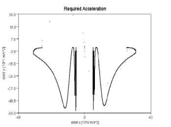
Figure 3.4: The strange attractor of the adaptively deformed “required responses”rn:= ¨qReq(n)(x:= ¨qReq1 ,y:=
¨
q2Req) of the adaptive RFPT-based controller in its nonconvergent regime for104control cycles [A. 1]
Figure 3.5: Excerpt (the lower part of Fig. 3.4) of the strange attractor of the adaptively deformed “required re- sponses”rn:= ¨qReq(n)(x:= ¨qReq1 ,y:= ¨qReq2 ) of the adaptive RFPT-based controller in its nonconvergent regime for 104control cycle: arrows denote the sequence of the consecutive points [A. 1]
Figure 3.6:The tracking error of the adaptive RFPT-based controller in its non-convergent regime [A. 1]
Figure 3.2 shows that in spite of the chaotic behavior of the control signal the trajectory tracking is acceptable, and the response error decreases in time (Figure 3.3). The chaotic behavior are clearly re- vealed by Figures 3.4 and 3.5. The connections of the arrows have considerable distances in Figure 3.5.
It means strong chattering. The tracking error, in a non-convergent regime of the Robust Fixed Point- based adaptive controller, is shown in Figure 3.6. In subsection 3.1.2, a simple chattering reduction method will be shown.
3.1.2 Chaos Reduction by Smoothing
In the SISO case [29], the amplitude of the observed small vibrations in the control signal was essentially determined by parameterK. For that case, necessarily a big number was chosen for parameterK.
In order to reduce these vibrations a sigmoid function was introduced for limiting the control signal so that instead ofrReq the limited signalrredReq =Ksσ(rReq
Ks
)was chosen with parameter0< Ks ≪ |K|.
The reason was that for “smallrReq” (i.e. for|rReq| ≪ |K|) no further deformation was necessary, so rredReq ≈rReq was guaranteed, and only the higher values (i.e. signals in the order of magnitude ofKs) were deformed/limited. Using that idea for a MIMO system with chattering reduction, the following equation can be written (3.5).
⃗h:=f⃗(⃗rn)−⃗rd, ⃗e:=⃗h/||⃗h||, B˜=Bσ(A||⃗h||)
⃗rn+1= (1 + ˜B)⃗rn+Ksσ(BK˜
Ks
)⃗e.
(3.5)
In the reduction the sigmoid functionσ(x) =1+x|x| was applied.
In the forthcoming simulationsKs = 15≪K = 106 was chosen in the control of the system defined in (3.2) and its rough model given in (3.3). Both Figs. 3.6 and 3.7 reveal that the chattering concerned only the componentq¨1Reqand that the chattering reduction considerably improved the trajectory tracking precision. Figures 3.8 and 3.9 provide convincing proof that the significantly reduced chattering must be practically tolerable since it results in smooth phase trajectory and only small relative fluctuation in the driving forces.
Figure 3.7:The tracking error of the adaptive RFPT-based controller in its nonconvergent regime with chattering reduction byKs= 15m/s2[A. 1]
Figure 3.8:The phase trajectory tracking of the adaptive RFPT-based controller in its nonconvergent regime with chattering reduction byKs= 15m/s2[A. 1]
Figure 3.9:The driving forces of the adaptive RFPT-based controller in its nonconvergent regime with chattering reduction byKs= 15m/s2[A. 1]
Figure 3.10: The “desired”, “realized”, and “required” accelerations of the adaptive RFPT-based controller in its nonconvergent regime with chattering reduction byKs= 15m/s2[A. 1]
Figure 3.11: The “desired”, “realized”, and “required” accelerations of the adaptive RFPT-based controller in its nonconvergent regime with chattering reduction byKs= 15m/s2(zoomed in excerpt) [A. 1]
Figure 3.12:The voting weights forA1= 10−7.5(black line),A2= 10−6.5(blue line), andA3= 10−5.5(green line) of the adaptive tuning [A. 1]
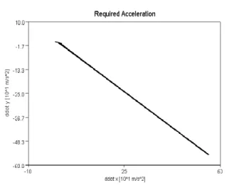
Figure 3.13: The strange attractor of the adaptively deformed “required responses”rn:= ¨qReq(n)(x:= ¨qReq1 ,y:=
¨
q2Req) of the adaptive RFPT-based controller in its nonconvergent regime for104 control cycles with chattering reduction byKs= 15m/s2[A. 1]
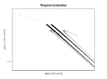
Figure 3.14: The strange attractor of the adaptively deformed “required responses”rn:= ¨qReq(n)(x:= ¨qReq1 ,y:=
¨
q2Req) of the adaptive RFPT-based controller in its nonconvergent regime for104 control cycles with chattering reduction byKs= 15m/s2(zoomed excerpt) [A. 1]
Figure 3.11 is a zoomed version of Figure 3.10. Those figures shows that in spite of the fact that there are little fluctuations present, the controller maintained its adaptive nature even in the non- convergence regime.
Figure 3.13 shows that the result practically becomes free of any chaos. Figure 3.14 shows the “fine structure” of this little “remnant chaos”. [A. 1]
3.1.3 A 3 DOF System
In the previous subsection it was shown that chaotic behavior can be handled with simple smoothing.
In the following part it will be investigated in the case of a 3 DOF system.
The motion equations for the 3DOF system is (4.1), and its schematic picture is shown in Figure 3.15. Thegeneralized coordinatesof the 3 DOF system are [A. 2]:
• q1(rad): rotation angle of the beam,
• q2(rad): rotation angle of the hamper at the top of the beam,
• q3(m): linear displacement of the cart’s body.
Thedynamic parametersare:
• mis the mass of the body, in top of the beam(kg)
• Mis the mass of the body of the “car”(kg)
• Lis the length of the beam(m)
• Θis the moment of inertia of the hamper with respect to its own mass center point(kg·m2) Thegeneralized forcesto be exerted by the controller are:
• Q1(N·m): torque at axle 1;
• Q2(N·m): torque at axle 2;
• Q3(N): force pushing the cart in the lateral direction,
furthermoregrepresents the gravitational acceleration. This model is just a rough initial model of the system. It is assumed that the hamper’s mass center point is located on its axle [A. 2].
For the RFPT method it is satisfactory to have some rough approximation of the dynamic parame- ters. Whenever the RFPT is applied for designing a “Model Reference Adaptive Controller (MRAC)”, also significant difference can be between the actual system’s parameters and that of the Reference Model to be imitated by the controlled system [59]. In the simulations carried out the MRAC solution was in- vestigated withactual system parametersasM= 30kg m= 10kg L= 2m,Θ= 20kg·m2,g= 10m/s2, whilethe reference modelhad the dynamic parameters asMˆ = 60kgmˆ = 20kgLˆ= 2.5m(also having effects on the dynamic behavior),Θˆ = 50kg·m2, andgˆ= 8m/s2. In the simulations it was assumed that the system’s response was observable as a noisy signal. ( In contrast to the other methods using various model-based estimators as Kalman filters, no any special assumption was necessary for the statistical nature of this observation noise, apart from the zero mean.) [A. 2]
(mL2+Θ) Θ mLcos(q1)
Θ Θ 0
mLcos(q1) 0 (m+M)
¨ q1
¨ q2
¨ q3
+ +
−mLgsin(q1) 0
−mLsin(q1) ˙q12
=
Q1 Q2
Q3
(3.6)
Figure 3.15: Sketch of the model used for the computation [A. 2]
3.1.4 Simulation Results and Chaos Patterns
In the simulations the following control parameter settings were used: Ks = 600,Kc= 7000,Bc=−1, andAcwas adaptively tuned in the case of necessity. Figures 3.36 and 3.17 display the trajectories and the phase trajectories of the controlled system revealing that the tracking in both spaces remained smooth and precise. Figure 3.18 reveals that besides the considerable parameter differences between the actual and the reference models significant observation disturbances were assumed. According to Figs. 3.19, 3.20, and 3.21 it can be stated that quite significant adaptive deformation was necessary for the imitation of the reference model but all the occurring accelerations are very close to each other that testifies the success of the adaptive controller. Figure 3.21 reveals the details of the adaptation mechanism showing that thereferenceand therecalculatedvalues are in each other’s close vicinity, i.e.
the “illusion” to be created by the MRAC controller was successful, too. Figure 3.20 displays an excerpt of Fig. 3.21 that clearly shows that thereferenceand therecalculated values (i.e. the cyan–yellow, the red–dark blue, and the magenta–light blue pairs) are closely in each other’s vicinity. The tracking
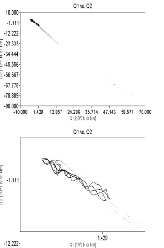
errors are displayed in Fig. 3.22. Figures 3.23-3.25 reveal the formation of the very much curbed chaos pattern in the exerted control forces.[A. 2]
Figure 3.16: The nominal (q1: black,q2: blue,q3: green lines) and the simulated trajectories (q1: cyan, q2: red,q3: magenta lines) [A. 2]
Figure 3.17: The nominal (q1: black,q2: blue,q3: green lines) and simulated (q1: cyan,q2: red,q3: magenta lines) phase trajectories [A. 2]
Figure 3.18: The exerted control torques (Q1: black,Q2: blue,Q3: green lines), and the noisy disturbance forces (Q1: cyan,Q2: red,Q3: magenta lines) [A. 2]
Figure 3.19: The second time-derivatives of the generalized coordinates (realized: q¨1: yellow,q¨2: dark blue,q¨3: light blue, kinematically desired:q¨1: cyan,q¨2: red,q¨3: magenta, nominal:q¨1: black,q¨2: blue,q¨3: green lines) [A. 2]
Figure 3.20: Theexerted(Q1: black,Q2: blue,Q3: green lines), therecalculated(Q1: yellow,Q2: dark blue,Q3: light blue lines), and thereference(Q1: cyan,Q2: red,Q3: magenta lines) (zoomed excerpt) [A. 2]
Figure 3.21: Theexerted(Q1: black,Q2: blue,Q3: green lines), therecalculated(Q1: yellow,Q2: dark blue,Q3: light blue lines), and thereference(Q1: cyan,Q2: red,Q3: magenta lines) [A. 2]
[A. 2]
Figure 3.22: The trajectory tracking error (q1: black,q2: blue,q3: green lines) [A. 2]
Figure 3.23: The projection of the generalized forces on theQ1-Q2plane with zoomed excerpts [A. 2]
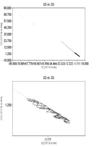
Figure 3.24: The projection of the generalized forces on theQ2-Q3plane with zoomed excerpts [A. 2]
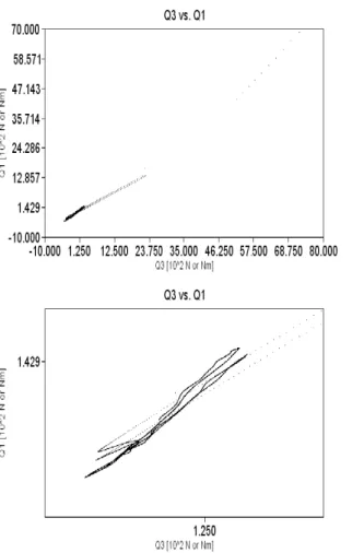
Figure 3.25: The projection of the generalized forces on theQ3-Q1plane with zoomed excerpts [A. 2]
3.2 Investigating Asymmetries in Chemical Systems
3.2.1 Challenges in Controlling Chemical Systems
Controlling Chemical Systems usually could be harder that of Classical Mechanical Systems. The usual problems can be summarized as follows:
1. Normally in Classical Mechanical Systems the control torque or force components can have pos- itive and negative values. In contrast to that the control actions in chemical systems correspond to adding dense reagents into tank reactor therefore they can have only positive values. It is im- possible to extract pure components from the mixture that could correspond to negative control actions. Therefore the action must be cut at zero whenever negative values would be desired by the controller. During such sessions the system remains without efficient control.
2. In Classical Mechanics the velocity can be positive and negative. In chemical systems negative concentrations do not have physical interpretation. Normally the analytical equations do not con- tain these restrictions and from purely mathematical point of view they could be applied by the controller even when not having physical relevance.
3. In the useful model the original equations have to be completed by these restrictions. If the con- centration reaches zero its time derivative cannot be negative. Consequently it is dangerous to
use big feedback terms because they may cause big concentrations of certain reagents which cannot be decreased quickly in the following session of the control process.
4. Normally the various components cannot be separately controlled. When a dense reagent is added to the system it automatically dilutes the other components while increases the concen- tration of the desired one. I referred to this effect asinput coupling. In the great majority of the literature this effect is completely neglected. I systematically investigated its effect in the struc- ture of the possible control strategies.
5. The structure of the RFPT-based adaptive method naturally allows the use of various derivatives for the control of various order or relative order physical systems. It is well known that the higher order derivatives are very noise-sensitive expressions. The idea naturally arose to use non-integer order ones for the purpose of adaptive control. The fractional order derivatives correspond to long system memory therefore their use can be interpreted as the application of certain noise filtering effect. A natural expectation also arose that due to the use of longer internal memory the cycle time of the adaptive controllers may be increased by the use of fractional order derivatives in the learning process. This would have practical significance whenever the cycle time of the available sensor is limited. The idea was investigated by simulations in the case of a chemical process.
During former investigations it was also observed that leaving the region of convergence not nec- essarily leads to the decay of the adaptive control. It trajectory tracking can remain precise at the cost of the appearance of big chattering in the control signal. In [29] simple method was successfully sug- gested for the reduction of this chattering. [A. 3].
3.2.2 The Particular Paradigms Under Consideration
The investigated system was the famousBrusselator Model of the Belousov-Zhabotinskii Reactionde- veloped by Prigogine and Lefever in 1968 [60].
3.2.3 RFPT-based Adaptive Control of the Brusselator Model
The portmanteau “Brusselator” introduced by J.J. Tyson in 1976 in [61] refers to theBrussels School of Thermodynamicsin which the first model ofchemical oscillationswere mathematically expounded.
In [62] the reactions described by (3.9) were used with assumedly constantAandB mole/Lconcen- trations. In the present paper its modification (3.10) is applied with the assumption that in a stirred reactor vessel of volumeV during a small time-intervalδt,δNAingress of the very dense reagentAof negligible volume is introduced that does not observably dilute the other reagents in the vessel. Sim- ilar assumption was made for reagentBthat led todecoupled control signalsasuA := δNV δtA ≥0and uB:= δNV δtB ≥0of dimension moleL·s . Since the moleculesX,Y,DandEare produced ofAandBin this approach replenishment of componentsAandBmust be satisfactory for control purposes. Since the time-derivatives of the first two equations of (3.10) containedA˙andB˙a 2nd order PID-type control was designed for thedesiredX¨dandY¨dvalues (exactly of the same form that was considered in the case of the coupled springs) that so provided thedesiredA˙d andB˙d by the use of whichuAanduBwere determined from the last two equations according to the available model [A. 3].
In the forthcoming simulations theexact parameterswere assumed to bek1= 1,k2= 1,k3= 1, and k4= 1whilethe approximate ones used by the controllerwerek˜1= 0.8,k˜2= 0.9,k˜3= 0.7, andk˜4= 0.6 of appropriate physical dimensions that comply with (3.10). The simulations made forΛ= 6/sfor the non-adaptive simple PID controller for large amplitude (0.5moleL ) oscillation in the nominal trajectory of frequencyω= 3/sprovided nice trajectory tracking but in it thephysically not interpretableuA<0,uB<0, A <0,B <0quantities also occurred. For getting rid of the physically not interpretable sessions (3.10) were completed with truncations for the negative values. This lead to completely unapplicable PID
control that allowed fast rate of increase in certain concentrations with considerable positive ingress rates, however, since the extraction of pure reactants were impossible the decreasing phases were left without active control with longuA≡0anduB≡0sessions. These asymmetries are the main barriers of the available control speed.On this reason the fast transients of the iterative learning that were not critical in the case of the mechanical system were carefully avoided in the case of the chemical reaction by setting thecycle time of the controller10msand the discrete time-resolution of the Euler integration to 1ms. Furthermore nominal trajectory of considerably smaller amplitudeH= 0.05moleL was considered for which the common PID controller provided useful results (Fig. 3.26). The results obtained for the adaptive counterpart of the controller for the same nominal motion are given in Fig. 3.27 for theadaptive parameter settingsKc= 600,Ks= 5moleL·s2,Bc =−1, andAc ∈ {1.67,5.27,16.67,52.70,166.67,527.05} × 10−5 moleL·s2. The adaptivity was switched on at t = 5swhen the rough initial transients were already damped by the common PID controller and further refinement of the tracking properties became actual.
The improvement in the tracking precision in the stabilized stage of the motion is evident [A. 3].
A→k1X, B+X→k2Y+D,
2X+Y →k33X, X→k4E. (3.7)
X˙ =k1A−k2BX+k3X2Y−k4X, Y˙ =k2BX−k3X2Y , A˙=−k1A+uA,B˙=−k2BX+uB.
(3.8)
Figure 3.26:Tracking error of the simple non-adaptive PID controller in the non-transient stage (forX: black and green lines, forY: blue and red lines) [A. 3]
Figure 3.27:Tracking of the adaptive controller (forX: black and green lines, forY: blue and red lines) [A. 3]
Figure 3.28 reveals the details of the adaptation mechanism [A. 3].
Figure 3.28: The “desired” (X: black,¨ Y¨: blue), adaptively deformed “required”(X: magenta,¨ Y¨: purple), and the realized(X: green,¨ Y¨: red) signals of the adaptive controller, and the control signals (uA: black,uB: blue) [A. 3]
3.2.4 Input Coupling in the Control of the Brusselator Model
In [62] the reactions described by (3.9) were used with assumedly constantAandB[
mole L
]concen- trations. (No any mechanism was detailed regarding the question how to keep these concentrations constant [A. 4].)
A→k1X, B+X→k2Y+D,
2X+Y →k33X, X→k4E (3.9)
that leads to the reaction equations as follows:
X˙ =k1A−k2BX+k3X2Y−k4X Y˙ =k2BX−k3X2Y
A˙=−k1A, B˙=−k2BX
(3.10)
in whichk1,k2,k3andk4are assumed to be constants. Presently we assume that the active volume of the CSTR isV[L], the actual concentrations of the reagents areA,B,X,Y, and at the inlets of reagentsA andBthe available concentrations areρA, andρB
[mole
L
], respectively. We also assume that the volumes are additive that (in the case of not very great concentrations) may be reasonable. We should like to simultaneously produce the nominalXN om(t)andYN om(t)concentrations by adding the reagentsA andBinto the reaction vessel, and if necessary, by egressing some amount of solution from the tank.
If the controller so operates that during timeδt δwA[L]of reagentAandδwB [L]of reagentBare pumped into the well stirred tank, furthermoreδV [L]mixture is egressed at the outlet the appropriate mole numbers and full volume after timeδtwill be as follows [A. 4]:
![Figure 3.1: Schematic figure explaining the formation of chaos for a 1 DOF system [A. 1]](https://thumb-eu.123doks.com/thumbv2/9dokorg/513976.40/17.918.305.651.126.576/figure-schematic-figure-explaining-formation-chaos-dof.webp)