THE EFFECT OF THE DEPENDENCE STRUCTURE ON RISK MEASURES
Edit Csizmás 1*, Edith Kovács 2
1 Department of Information Technology, GAMF Faculty of Engineering and Computer Science, John von Neumann University, Hungary
2 Department of Differential Equations, Budapest University of Technology and Economics, Hungary https://doi.org/10.47833/2021.3.CSC.004
Keywords:
elliptical copula Archimedean copula risk measure
dependence structure conditional independence Article history:
Received 30 Oct 2021 Revised 20 Nov 2021 Accepted 25 Nov 2021
Abstract
After the financial crisis of 2008, the goodness of mathematical models became strongly questionable. One of the main targets of the attacks was the application of the Gaussian copula. The risk measures proposed were the Value at Risk (VaR) and Conditional Value at Risk (CVaR). We show how the values of these risk measures are influenced by different kinds of dependency structures, which are modelled by different copulas. Archimedean copulas are used for modelling tail dependences and asymmetrical dependencies. We present their impact on the portfolio’s probability distribution. We explain why in the case of multivariate distribution Gauss Copula and Student copula are good alternatives. We also show how conditional independence can be used for giving more flexible approximations.
We illustrate on simulated and also on real data the impact of the dependence structure on VaR and CVaR.
In memoriam Professor Tibor Vajnai (1961-2020)
1 Introduction
Uncertainty is present in every future accomplished event therefore all of our actions are containing some risk in them. If the uncertainty can be modelled via a probability distribution, then the risk can be quantified also in terms of probability.
People mostly agree to take expected returns as a measure of the performance of a portfolio, however, there is no consensus which risk measure captures better the risk. In the seminal work of Markovitz [1], the variance is considered as a risk measure. This can be a good choice when the probability distribution is Normal or at least symmetrical.
Value at Risk (VaR) has become a very popular risk measure since it was introduced by the Bank of International Settlements and USA regulatory agencies in 1988, and also was recommended as a standard by the Basel Committee. VaR was criticized for two reasons. Firstly, because VaR is not a coherent risk measure as it was defined by Artzner et al [2], it is not a convex measure of risk thus it may have many local extrema, which may cause technical problems when optimizing a portfolio. Secondly, it gives a percentile of loss distribution and does not provide a picture of the possible losses in the tail [3]. Other risk measures were proposed, one of them which also will be discussed in our paper is Conditional Value at Risk (CVaR on the other name Expected Shortfall ES). CVaR depends on the “fatness” of the tail of the distribution. An overview of CVaR
* Corresponding author. Tel.: +36 76 516 444 fax: +36 76 516 399 E-mail address: csizmas.edit@gamf.uni-neumann.hu
can be found in [4]. Rockafellar and Urysaev [5], [6] proposed a minimization formulation that usually results in a convex or linear problem.
In practice, however, no matter which type of risk measure will be adopted, the validity of its estimation depends on the accuracy of the joint probability distribution of the asset returns.
Gaussian distributions were commonly used in multivariate probability distribution modelling, because of the efficient algorithms used in calibration and simulation. One of the obvious disadvantages is its symmetry which would imply that the probability of losses is the same as the probability of gains. Studies suggest that the assets exhibit stronger comovements during a crisis [7], [8]. One way to overcome this is the use of mixtures of distributions. Copulas were suggested by Zhu and Fukushima [4] within the worst-case robust scenario.
The present paper aim is to highlight the impact of the dependency structure on VaR and CVaR.
The paper is structured as follows. In Section 2 we introduce briefly the theoretical background. In Section 3 we simulate different portfolios and discuss the different risk measures.
Then in Section 4, we provide a numerical example of real data.
2 Theoretical background
In this section, the definitions of the concepts and the theorems which we use in this paper are given.
2.1 The copula method
The copulas arose from the theory of metric function and were introduced by Sklar in [9].
Copulas are popular because they make possible the separate modelling of the marginal probability distribution and the dependence between them. This way multivariate probability distributions can be modelled in a much more flexible way.
The general definition of a 𝑑-dimensional copula is the following [10]:
Definition 1
𝐶: [0,1]𝑑→ [0,1] function is 𝑑-copula (𝑑-dimensional copula), if it has the following properties:
(i) ∀𝑢𝑖 ∈ [0,1], 𝐶(𝑢1, … , 𝑢𝑑) = 0, if there is at least one 𝑢𝑖 = 0, (ii) ∀𝑢 ∈ [0,1], 𝐶(1, … ,1, 𝑢, 1, … ,1) = 𝑢,
(iii) ∀ 𝑢𝑖 ∈ [0,1], 𝐶(𝑢1, … , 𝑢𝑑) ≥ 0, 𝑑-increasing.
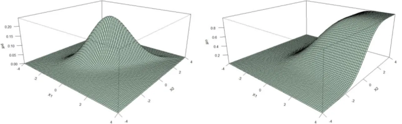
The probability density function (PDF) and the cumulative density function (CDF) of a two- dimensional copula are presented in Figure 1.
Figure 1. The CDF and PDF of the two-dimensional Gumbel copula (𝜃 = 2 with uniform marginals 𝑢1, 𝑢2)
Now let us explain in a geometrical way the definition of a copula which in fact is a cumulative probability density function of a multivariate random vector with a 1-dimensional uniform marginal probability distribution. To give a better intuition for the definition, we explain the definition in the two-dimensional case. On the right-hand side of Figure 1 the yellow line illustrates
the property (i) of Definition 1, the blue line illustrates the property (ii) of Definition1. The property (iii) expresses that the volume under the copula is positive.
The following theorem published in 1959 [11] can be regarded as the central theorem of copula theory.
Sklar’s theorem
Let 𝐹 be an 𝑛-dimensional joint distribution function with 1-dimensional marginals 𝐹1,…, 𝐹𝑑, then exist a copula function 𝐶 such that
𝐹(𝑥1, … , 𝑥𝑑) = 𝐶(𝐹1(𝑥1), … , 𝐹𝑑(𝑥𝑑)) (1) for all real 𝑑-tuples (𝑥1, … , 𝑥𝑑).
If each marginal is continuous, then the 𝐶 is unique.
If we suppose that 𝐶 and 𝐹𝑖 in formula (1) are differentiable then the joint probability density function 𝑓(𝑥1, . . 𝑥𝑑) can be expressed as follows:
𝑓(𝑥1, … , 𝑥𝑑) = 𝑐(𝐹1(𝑥1), … , 𝐹𝑑(𝑥𝑑) ) ∙ 𝑓(𝑥1) ∙ … ∙ 𝑓(𝑥𝑑) . (2) Using the 𝐹𝑖(𝑥𝑖) = 𝑢𝑖 transformation we get the copula density function 𝑐(𝑢1, … , 𝑢𝑑):
𝑐(𝑢1, … , 𝑢𝑑) =𝜕𝑑𝐶(𝑢1,…,𝑢𝑑)
𝜕𝑢1…𝜕𝑢𝑑 .
The probability density function (PDF) and the cumulative density function (CDF) of a two- dimensional Gumbel copula with normal marginals are presented in Figure 2.
Figure 2. The CDF and PDF of the two-dimensional Gumbel copula (𝜃 = 2 with normal marginals 𝜇 = 0, 𝜎 = 1)
In our present experiments, we work with the Gauss and Student elliptical copulas and with Clayton, Gumbel and Frank Archimedean copulas.
The Gaussian and Student’s 𝑡-copula are elliptical copulas so both of them are radially symmetric. These copulas can be described by the following formula [12]:
𝐶(𝑢1, … , 𝑢𝑑) = 𝐹(𝐺−1(𝑢1), … , 𝐺−1(𝑢𝑑)), (𝑢1, . . . , 𝑢d) ∈ [0,1]𝑑,
wherein the case of Gauss copula 𝐹 = 𝛷𝑅 is the multivariate Gauss distribution corresponding to a correlation matrix 𝑅 and 𝐺−1= 𝜙−1 is an inverse function of the univariate standard normal distribution; in the case of Student copula 𝐹 = 𝑡𝑅,𝜈 is the multivariate Student distribution and 𝐺−1= 𝑡𝜈−1 is an inverse function of the univariate standard 𝑡-distribution with 𝜈 degrees of freedom.
Besides the elliptical copulas, the Archimedean copulas are also very popular in multivariate probability distribution modelling.
The two-dimensional Archimedean copulas were introduced in Genest and Mac [13], [14].
Their definition was then easily extended to the multivariate case.
First, the so-called generator function has to be defined.
The function 𝜑: [0; 1] ⟶ [0; ∞] which fulfils the following properties is called generator function:
𝜑 continuous,
𝜑 is strictly decreasing and 𝜑(1) = 0, 𝜑(∞) = 0,
𝜑[−1] is completely monotonic on [0; ∞],
where 𝜑[−1] is the pseudoinverse [10] defined as follows:
𝜑[−1](𝑡) = {𝜑−1(𝑡) , 0 ≤ 𝑡 ≤ 𝜑(0) 0, 𝜑(0) < 𝑡 ≤ ∞
Now, having the general definition of the generator function, the multivariate Archimedean copula can be defined in the following way.
Definition 2
The copulas defined by using the generator function 𝜑
𝐶(𝑢1, … , 𝑢𝑑) = 𝜑[−1](𝜑(𝑢1), … , 𝜑(𝑢𝑑)) are called Archimedean copulas (Table 1).
The Archimedean copula usually depends on one or two parameters which can be calculated based on Kendall’s tau. In this paper, we will use Clayton, Gumbel and Frank copula.
Table 1. The generators of the Archimedian Copulas [10]
𝜑𝜃(𝑡) 𝜃 Properties
Clayton 1
𝜃(𝑡−𝜃− 1) [−0, ∞)/{0} strict Gumbel (− ln 𝑡)𝜃 [1, ∞) strict
Frank − ln𝑒−𝜃𝑡− 1
𝑒−𝜃− 1 (−∞, ∞)/{0} strict
radially symmetry The generator of the copula is strict if 𝜑(0) = ∞ [10].
These copulas can describe different kinds of dependencies. Clayton copula can model the stronger lower tail dependence, Gumbel copula the stronger upper tail dependence, and Frank copula, which in contrast with the former two this is a symmetrical copula without tail-dependence.
2.2 Measures of risk
In the present paper, we will investigate the impact of the dependence structure on two risk measures.
Value at Risk (VaR) and Conditional Value at Risk (CVaR) have become popular risk measures in portfolio risk management. Important results related to VaR can be found in [15], and related to CVaR in [6], [16], [17].
Let us introduce the definition of these two risks “measures”. It is worth noting here that only CVaR is a risk measure. Although VaR expresses risk it does not fulfil the subadditivity property therefore in rigorous terminology it is not a measure.
Table 2. The formulas of the Value at Risk and the Conditional Value at Risk Risk in lower tail Risk in upper tail
VaR 𝑉𝑎𝑅𝛼𝐿 = 𝐹−1(𝛼) 𝑉𝑎𝑅𝛽𝑈= 𝐹−1(1 − 𝛽)
CVaR 𝐶𝑉𝑎𝑅𝛼𝐿= ∫ 𝑡𝑓(𝑡)𝑑𝑡
𝑉𝑎𝑅𝛼𝐿
−∞
𝐶𝑉𝑎𝑅𝛽𝑈= ∫ 𝑡𝑓(𝑡)𝑑𝑡
∞ 𝑉𝑎𝑅𝛽𝑈
VaR and CVaR are commonly related to the loss distribution, we make an extension of these and examine their values on both tails of the probability distribution of loss or gain.
Shortly speaking from a probability theoretical point of view VaR is a quantile, which corresponds to a given probability, whereas CVaR is a conditional expectation calculated in the tail of the probability distribution.
Since we are not only interested in risk but also in profit, we consider extreme values on both sides (Figure 3 and Table 2). In other words, not only low yields can be risky, but high yields too, such as the amount of water in rivers, should be considered yields, then when two rivers meet, too high yields can cause flooding. Therefore, copulas are often used in hydrology also [18].
Figure 3. Value at Risk and Conditional Value at Risk on bottom and top
3 Exploring the impact of the dependence structure on the risk measure of a simulated portfolio
This part is based on simulated data. The aim of this part is on the one hand to exhibit some of the good properties of the Gauss copula which many times are ignored, on the other hand, we will illustrate the impact of the copula type on the risk of a portfolio calculated. It is important to note here that the risk is calculated based on a univariate probability distribution of a random variable 𝑆 which is a sum of random variables, which correspond to the returns of the component assets.
Dealing with risk is not important only for portfolios, the same problem appears also in the case of floods caused by two or more rivers.
Many papers are written on related topics, most of them are using copulas in the simulation of future data and are concerned with giving accurate forecasting [19]. In fact, most of the papers use copulas for modelling the residuals in the case of time series.
The aim of our paper is to give insight to the impact of the dependence structure on the VaR and CVaR risk measures.
3.1 The role of the marginals in modelling fat tails, and asymmetric probability distributions
In this subsection, we present three cases of two-dimensional joint probability distributions.
All three are generated by Gaussian copulas. The first one (Figure 4a) has both of the marginal probability distributions Gaussian, the second one (Figure 4b) has one of the marginal probability distribution exponential and the other one normal, the third one has both of them exponential (Figure 4c).
Figure 4. Gauss copula (𝜚 = 0.8) with a) two normal (𝜇 = 3, 𝜎 = 1), b) normal (𝜇 = 3, 𝜎 = 1) and exponential (𝜆 =1
3), c) two exponential (𝜆 =1
3) marginals (𝑁 = 2000) 𝑉𝑎𝑅𝛽
𝐶𝑉𝑎𝑅𝛽
𝑉𝑎𝑅𝛼
𝐶𝑉𝑎𝑅𝛼
𝛼 𝛽
a) b) c)
In Figure 4b the asymmetry of the joint probability distribution and the strong lower tail dependence can be observed. In Figure 4c these properties skewness and also the strong lower dependence can be observed. In Figure 4 the illustrations exhibit the role of the marginal distribution, in the case of the Gaussian copula.
These examples show that strong tail dependence and asymmetry can be achieved with Gaussian copula also, by using the appealing property that arbitrary marginal probability distributions can be chosen.
3.2 The role of the copula in joint probability distributions modelling and its impact on the risk measures
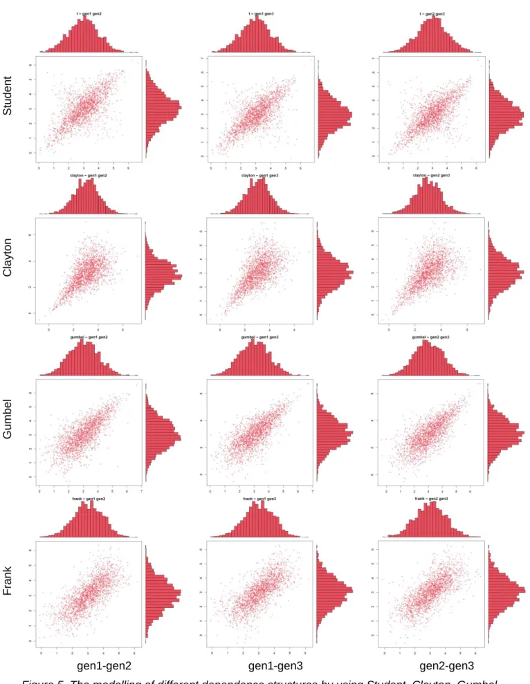
In this experiment, the reference data set was generated with a 3-dimensional normal copula by first taking all marginals as normally distributed and then working with one exponential and the other two normally distributed. In this experimental case, we took the same ϱ=0.8 correlation coefficient between all the marginals. Then in the first subsection, different copulas were fitted to the reference data preserving the normal marginals. For modelling of different dependence structures Student, Clayton, Gumbel, Frank copulas were proposed (Figure 5). The parameters of the copulas were adjusted to the same ϱ=0.8 (by fitting different copulas to the sample generated of the normal copula).
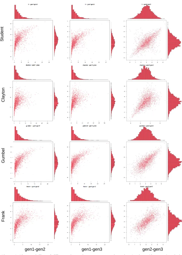
In the second subsection, one exponential and two normal marginals are chosen. The two- dimensional marginals are presented (Figure 6).
The last subsection discusses the effect of the copula type on the risk measures (Figure 7).
3.2.1 The effect of the copula
In this subsection, the joint distribution was generated by four copula types and the same normal marginal distributions. In Figure 5 the effect of the copula type on the probability distribution is shown. In one row the two-dimensional projection of the points simulated from a given third- order copula (Student in the first row, Clayton in the second row, Gumbel in the third row and Frank in the last row) and normal marginals is illustrated. In the first row, the points are in an elliptical shape because of the 𝑡-copula, in the second row the lower tail dependence of the Gumbel copula is illustrated, in the third row the upper tail dependence of the Clayton copula is revealed and in the last row Frank copula is illustrated, without any tail dependence. In each row, we can observe the effect of a different copula. In the first row the points are in an elliptical shape because of the 𝑡- copula, in the second row the lower tail dependence of the Gumbel copula is illustrated, in the third row the upper tail dependence of the Clayton copula is revealed and in the last row Frank copula is illustrated, without any tail dependence.
3.2.2 The effect of different copula types combined with the effect of different marginals
The simulations in this part exhibit, the effect of the copula type and the effect of the three marginals, one exponential and two Gaussians at the same time. For a given copula the bivariate projections (marginals) are illustrated in the same row (Figure 6).
In the case of 𝑡-copula, we chose for all three dependencies between the marginals the same 𝜚 = 0.8. In general, a covariance or correlation matrix, which defines a multivariate normal or a 𝑡-copula may contain different values. This makes the normal and 𝑡-copula much more flexible than the multivariate Archimedean copulas, in higher dimensions. Therefore, this is a very appealing property of the normal and 𝑡-copula. By using this property, we can model at the same time a multivariate distribution with different kinds of dependencies between its components. The only constraint for the correlation matrix is to be positive semidefinite.
Using the simulations presented in this subsection and the previous one, a study on the VaR and CVaR is conducted in the next part.
Student ClaytonGumbelFrank
gen1-gen2 gen1-gen3 gen2-gen3
Figure 5. The modelling of different dependence structures by using Student, Clayton, Gumbel, Frank copulas and marginals generated from a Gauss copula (𝜚 = 0.8) with three normal
(𝜇 = 3, 𝜎 = 1) marginals (𝑁 = 2000)
Student ClaytonGumbelFrank
gen1-gen2 gen1-gen3 gen2-gen3
Figure 6. The modelling of different dependence structures by using Student, Clayton, Gumbel, Frank copulas and marginals generated from a Gauss copula (𝜚 = 0.8) with exponential (𝜆 =1
3) and two normal (𝜇 = 3, 𝜎 = 1) marginals (𝑁 = 2000)
3.2.3 The effect of dependency structure on risk measures
Based on the simulations in subsections 3.2.1 and 3.2.2 we illustrate the VaR and CVaR related to the sum of the three marginals. We have to note here that the correlation coefficient used for the multivariate student copula for defining the correlation matrix, and for the expression of the parameters of the Archimedean copulas is relatively high 𝜚 = 0.8.
Looking at Figure 7a we can observe the effect of different copula types on the portfolio, having the same marginals. It can be observed that in the case of Clayton copula we have a lower VaR (UVaR) and CVaR (UCVaR), in the case of Gumbel copula we have a higher Var (LVar) and lower CVaR (LCVaR). Figure 7b exhibits also what a difference it makes when we have different kinds of marginals. The mean value, the upper VaR and the upper CVaR are much higher than in the previous case. The typical effect of the Clayton copula and Gumbel copula is much easier to be observed.
Three normal marginals An exponential and two normal marginals
Figure 7. The VaR and CVaR of the portfolio
0 5 10 15 20 25
X t clayton gumbel frank
a) rho=0.8
mean L VaR U VaR
L CVaR U CVar
0 5 10 15 20 25
X t clayton gumbel frank
b) rho=0.8
0 5 10 15 20 25
X t clayton gumbel frank
c) rho=0.95
0 5 10 15 20 25
X t clayton gumbel frank
d) rho=0.95
0 5 10 15 20 25
X t clayton gumbel frank
e) rho=0.1
0 5 10 15 20 25
X t clayton gumbel frank
f) rho=0.1
Another interesting question is how 𝜚's value influences the differences between the effects of copulas. If the value of 𝜚 is close to 1 then a very close linear dependency exists between the random variables, this causes that all the simulations will be close to each other (Figure 7c and d).
In the case when the value of 𝜚 is very close to 0 every copula gets closer to the independence copula, this way the simulation results also getting closer. It is also interesting to note that in the case of independence (low dependence) the interval between the UVaR and LVaR is more narrow, which is absolutely in line with the aim of portfolio diversification (Figure 7e and f), in order to decrease the risk of the portfolio.
4 Exploring the effect of the dependence structure in risk characterization on real time-series data
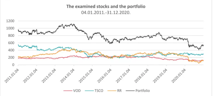
This part contains an illustration of the role of dependency, encoded by the copula, on real data which was downloaded from Yahoo Finance (https://finance.yahoo.com/). We consider a portfolio that consists of the prices of three stocks registered weekly for 10 years (from 04.01.2011 to 31.12.2020). The three stocks (Tesco PLC, Vodafone Group Plc, Rolls-Royce Holdings plc) is from the FTSE100. The time horizon is 𝑇 = 2521. The graphs of the three-time series and their sum are illustrated in Figure 8.
Figure 8. The time series of the stocks
It can be easily observed that these time series are not stationary firstly because they contain a trend. To transform them into time series without trend the following transformation called log return is introduced:
𝑟𝑡= 𝑙𝑛 𝑝𝑡
𝑝𝑡−1 .
We are interested in the log return of the portfolio, denoted by 𝑅𝑡, which is defined as follows 𝑅𝑡 = 𝑙𝑛 𝑆𝑡
𝑆𝑡−1 , where 𝑆𝑡 denotes the value of the portfolio at time 𝑡.
The log return of the portfolio can be approximated by a weighted sum of the log-returns of the stocks [19].
From the practical point in literature, many times the weights are substituted by 1
𝑚, in the case of 𝑚 stocks. One of the reasons for doing this is that weights should stay constant in time, in order to get a picture of the portfolio’s riskiness.
0 200 400 600 800 1000 1200
The examined stocks and the portfolio 04.01.2011.-31.12.2020.
VOD TSCO RR Portfolio
In the following the log return of the portfolio is substituted with its approximation the sum of the log-returns of the stocks involved [20].
Now the random variables are the log-returns of the three assets, expressed in percentages.
These time series are shown in Figure 9.
We want to characterize the risk by upper and lower VaR and upper and lower CVaR, in the case of the best fitting copulas from different copula families.
The next procedure is used:
Step1 Finding good marginal probability distributions. We fit the marginal empirical data univariate marginal probability distributions. These probability distributions are used throughout the experiment.
Step2 Finding the best copula from a copula family.
The empirical marginals are transformed into uniform marginals.
The three-dimensional empirical copula having uniform marginal is used to fit it the best copula from a given family (normal, t, Clayton, Gumbel, Frank). As a result, we get the parameters that characterize the best copula in each family.
Step3 The uniform marginals are substituted by the continuous marginals obtained in Step1.
Step4 For every type of copula (with the parameter chosen in Step2), with the marginal obtained in Step1 we simulate 10 000 three-dimensional data points.
Step 5 We calculate based on each data point the value of the equally weighted portfolio.
Step 6 We evaluate the upper and lower VaR and CVaR.
Figure 9. The yields of the stocks and their portfolio
Before the results are presented let us make some observations. In this case, the normal and the Student’s 𝑡-copula have not only one correlation coefficient like in the 3-rd section. Each pair has a different correlation coefficient. This shows again the flexibility of a multivariate Student or Gauss in opposition with an Archimedean copula, with only one parameter (or two, three in certain
-20 -10 0 10 20
VOD
-20 -10 0 10 20
TSCO
-50 -40 -30 -20 -10 0 10 20 30 40 50
RR
-50 -40 -30 -20 -10 0 10 20 30 40 50
Portfolio
cases) also in higher dimension (Table 3). To all the univariate marginals the 𝑡-distribution gives the best fitting with 3.40, 2.66 and 1.81 degrees of freedom.
Another concept that is explored here is conditional independence. We illustrate here the basic idea in the case of three random variables.
Let us suppose that we have three random variables 𝑋, 𝑌, 𝑍.
By using the chain formula, we have
𝑓𝑋𝑌𝑍(𝑥, 𝑦, 𝑧) = 𝑓𝑋(𝑥)𝑓𝑌|𝑋(𝑦|𝑥)𝑓𝑍|𝑋𝑌(𝑧|𝑥, 𝑦).
Now let us suppose that we want to approximate 𝑓𝑋𝑌𝑍(𝑥, 𝑦, 𝑧) with a probability distribution, which encodes that X and Z are independent given 𝑋. In this case the last factor will be
𝑓𝑍|𝑋𝑌(𝑧|𝑥, 𝑦) = 𝑓𝑍|𝑌(𝑧|𝑦) therefore
𝑓𝑋𝑌𝑍(𝑥, 𝑦, 𝑧) = 𝑓𝑋(𝑥)𝑓𝑌|𝑋(𝑦|𝑥)𝑓𝑍|𝑌(𝑧|𝑦)
which can be expressed by applying the formulas of conditional probability densities as:
𝑓𝑋𝑌𝑍𝑎𝑝𝑝(𝑥, 𝑦, 𝑧) =𝑓𝑋𝑌(𝑥,𝑦)∙𝑓𝑌𝑍(𝑦,𝑧)
𝑓𝑌(𝑦) .
Now by using formula (2), we can express all the densities by using copulas:
𝑐𝑋𝑌𝑍𝑎𝑝𝑝(𝑢, 𝑣, 𝑤) = 𝑐𝑋𝑌(𝑢, 𝑣) ∙ 𝑐𝑌𝑍(𝑣, 𝑤) where 𝑢 = 𝐹𝑋(𝑥), 𝑣 = 𝐹𝑌(𝑦), 𝑣 = 𝐹𝑍(𝑧).
Table 3. The parameters of the fitted copulas copula type parameters
CI t(0.29;0.31)-t(6.56;5.22) normal rho(0.29;0.3;0.25) t rho(0.23;0.24;0.21) df(2) clayton alpha(0.33)
gumbel alpha(1.2)
frank alpha(1.65)
We will use only two of the three pairs of marginal probability distributions. We use those with the highest Kendall. It is proven that this one will give the best fitting from this kind of approximations. This type of copula has higher flexibility than the multivariate Archimedean copulas. In the conditional copula case, the copulas involved may have different types of nonlinear dependencies at the same time. Multivariate Gauss copula and 𝑡-copula are also flexible because they allow different types of dependencies at the same time. However, these dependencies are linear dependencies. Exploiting conditional independence, we can use in modelling even two different families (in the three-variable case).
Another idea that is explored here is conditional independence. We want to use only two of the three pairs of marginal probability distributions. We use those with the highest Kendall (Table 4). After this, only two 2-dimensional copulas will be used for modelling. This supposes that we use a conditional independence relation. This type of copula has higher flexibility than the multivariate Archimedean copulas. In the conditional copula case, the copulas involved may have different types of nonlinear dependencies at the same time. Multivariate Gauss copula and t-copula are also flexible because they allow different types of dependencies at the same time. However, these dependencies are linear dependencies. Exploiting conditional independence, we can use in modelling even two different families (in the three-variable case).
Table 4. The Kendall-𝜏matrix of the stocks
VOD TSCO RR
VOD 1 0.188 0.201
TSCO 0.188 1 0.168
RR 0.201 0.168 1
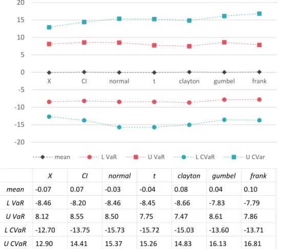
The differences between Risk measures for different types of copulas are presented in Figure 10. The copula, which involves conditional independence, is denoted as the CI copula.
X CI normal t clayton gumbel frank
mean -0.07 0.07 -0.03 -0.04 0.08 0.04 0.10 L VaR -8.46 -8.20 -8.46 -8.45 -8.66 -7.83 -7.79
U VaR 8.12 8.55 8.50 7.75 7.47 8.61 7.86
L CVaR -12.70 -13.75 -15.73 -15.72 -15.03 -13.60 -13.71 U CVaR 12.90 14.41 15.37 15.26 14.83 16.13 16.81
Figure 10. The VaR and CVaR of the portfolio
The copulas with the highest log-likelihood value out of a family are represented in Table 5.
In this application, the best fitting copula is the one that involves conditional independence. The explanation of this is that different pairs involved have different types of dependence, t(0.29;0.31)- t(6.56;5.22), which cannot be modelled by correlation.
Table 5. The log-likelihood of the copula fit evaluated at a given value of the parameters
CI normal t clayton gumbel frank
loglik 290.83 268.63 90.29 223.33 257.88 242.44
-20 -15 -10 -5 0 5 10 15 20
X CI normal t clayton gumbel frank
VOD-TSCO-RR
mean L VaR U VaR L CVaR U CVar
5 Conclusion
The aim of the paper was to illustrate the impact of the modelling of the multivariate probability distribution on the risk. We highlighted that heavy tails can be caused not only by using copulas with tail dependence, it may also be caused by the marginals used. The paper shows how the dependence expressed in terms of copulas has different kinds of impacts on risk measures.
We conducted different experiments in order to illustrate different aspects of dependence. We illustrate these in the three-dimensional case to give a good intuition to the reader. We drew attention to the fact that Gaussian and Student copulas are capable to encode different types of dependencies at the same time, this way these are more flexible than Archimedean copulas.
However, Archimedean copulas can model unsymmetrical dependence and tail dependence.
When we get a good approximation by exploiting the conditional independence relation, then we can use even more types of copulas for the pairs of marginals, at the same time. In fact, this stays at the root of using vine copulas in modelling multivariate copulas. On a real data set consisting of a portfolio with three equally weighted assets, the effects of different copulas used for the dependence modelling is presented. Moreover, we showed that in this case, the approximation based on conditional independence gives an even better approximation of the joint copula. In summary, we showed the importance of the modelling of the joint probability distribution by modelling the dependence structure separately from marginals to get accurate risk estimations.
Acknowledgment
This research is supported by EFOP-3.6.1-16-2016-00006 "The development and enhancement of the research potential at John von Neumann University" project. The Project is supported by the Hungarian Government and co-financed by the European Social Fund.
References
[1] H. Markowitz, “Portfolio Selection,” J. Finance, vol. 7, no. 1, pp. 77–91, 1952, doi: 10.2307/2975974.
[2] P. Artzner, F. Delbaen, J.-M. Eber, and D. Heath, “Coherent Measures of Risk,” Math. Finance, vol. 9, no. 3, pp. 203–228, Jul. 1999, doi: 10.1111/1467-9965.00068.
[3] G. Szegö, “Measures of risk,” Eur. J. Oper. Res., vol. 163, no. 1, pp. 5–19, May 2005, doi:
10.1016/j.ejor.2003.12.016.
[4] S. Zhu and M. Fukushima, “Worst-Case Conditional Value-at-Risk with Application to Robust Portfolio Management,” Oper. Res., vol. 57, no. 5, pp. 1155–1168, 2009.
[5] S. Uryasev and R. T. Rockafellar, “Conditional Value-at-Risk: Optimization Approach,” in Stochastic Optimization: Algorithms and Applications, vol. 54, S. Uryasev and P. M. Pardalos, Eds. Boston, MA:
Springer US, 2001, pp. 411–435. doi: 10.1007/978-1-4757-6594-6_17.
[6] R. T. Rockafellar and S. Uryasev, “Conditional value-at-risk for general loss distributions,” p. 29, 2002.
[7] A. Ang and J. Chen, “Asymmetric correlations of equity portfolios,” J. Financ. Econ., vol. 63, no. 3, pp.
443–494, Mar. 2002, doi: 10.1016/S0304-405X(02)00068-5.
[8] L. Hu, “Dependence patterns across financial markets: a mixed copula approach,” Appl. Financ. Econ., vol. 16, no. 10, pp. 717–729, Jun. 2006, doi: 10.1080/09603100500426515.
[9] M. Sklar, “Fonctions de repartition an dimensions et leurs marges,” Publ Inst Stat. Univ Paris, vol. 8, pp. 229–231, 1959.
[10] R. B. Nelsen, An Introduction to Copulas, 2nd ed. New York: Springer-Verlag, 2006. doi: 10.1007/0- 387-28678-0.
[11] A. Sklar, “Random variables, joint distribution functions, and copulas,” Kybernetika, vol. 9, no. 6, pp.
449–460, 1973.
[12] J.-F. Mai and M. Scherer, Simulating Copulas: Stochastic Models, Sampling Algorithms, and Applications, 2nd ed., vol. 06. WORLD SCIENTIFIC, 2017. doi: 10.1142/10265.
[13] C. Genest and J. MacKay, “The Joy of Copulas: Bivariate Distributions with Uniform Marginals,” Am.
Stat., vol. 40, no. 4, pp. 280–283, 1986, doi: 10.2307/2684602.
[14] C. Genest and R. J. MacKay, “Copules archimédiennes et familles de lois bidimensionnelles dont les marges sont données,” Can. J. Stat. Rev. Can. Stat., vol. 14, no. 2, pp. 145–159, 1986, doi:
10.2307/3314660.
[15] E. Wipplinger, “Philippe Jorion: Value at Risk – The New Benchmark for Managing Financial Risk: 3rd Edition, ISBN 0-07-146495-6, McGraw–Hill, 2007, 602 pages, approx. 120 CHF (hardcover),” Financ.
Mark. Portf. Manag., vol. 21, no. 3, pp. 397–398, Sep. 2007, doi: 10.1007/s11408-007-0057-3.
[16] G. Ch. Pflug, “Some Remarks on the Value-at-Risk and the Conditional Value-at-Risk,” in Probabilistic Constrained Optimization: Methodology and Applications, S. P. Uryasev, Ed. Boston, MA: Springer US, 2000, pp. 272–281. doi: 10.1007/978-1-4757-3150-7_15.
[17] R. T. Rockafellar and S. Uryasev, “Optimization of conditional value-at-risk,” J. Risk, vol. 2, no. 3, pp.
21–41, 2000, doi: 10.21314/JOR.2000.038.
[18] S. Naz, M. Ahsanuddin, S. Inayatullah, T. A. Siddiqi, and M. Imtiaz, “Copula-Based Bivariate Flood Risk Assessment on Tarbela Dam, Pakistan,” Hydrology, vol. 6, no. 3, p. 79, Aug. 2019, doi:
10.3390/hydrology6030079.
[19] P. Miskolczi, “Comparison of Risk Calculation Based on Historical Simulation and the Copula Function,” Public Finance Q., vol. 63, no. 1, pp. 80–95, 2018.
[20] P. Miskolczi, “Note on simple and logarithmic return,” Appl. Stud. Agribus. Commer., vol. 11, no. 1–2, pp. 127–136, Jun. 2017, doi: 10.19041/APSTRACT/2017/1-2/16.