On the solvability of the periodically forced relativistic pendulum equation on time scales
Pablo Amster
B, Mariel Paula Kuna and Dionicio P. Santos
Departamento de Matemática, Facultad de Ciencias Exactas y Naturales, Universidad de Buenos Aires & IMAS-CONICET, Ciudad Universitaria, Pabellon I (1428), Buenos Aires, Argentina
Received 30 May 2020, appeared 3 November 2020 Communicated by Paul Eloe
Abstract. We study some properties of the range of the relativistic pendulum opera- tor P, that is, the set of possible continuous T-periodic forcing terms pfor which the equation Px = p admits a T-periodic solution over a T-periodic time scaleT. Writ- ing p(t) = p0(t) +p, we prove the existence of a nonempty compact interval I(p0), depending continuously on p0, such that the problem has a solution if and only if p∈ I(p0)and at least two different solutions whenpis an interior point. Furthermore, we give sufficient conditions for nondegeneracy; specifically, we prove that ifTis small then I(p0)is a neighbourhood of 0 for arbitrary p0. The results in the present paper improve the smallness condition obtained in previous works for the continuous case T=R.
Keywords:relativistic pendulum, periodic solutions, time scales, degenerate equations.
2020 Mathematics Subject Classification: 34N05, 34C25, 47H11.
1 Introduction
The T-periodic problem for the forced relativistic pendulum equation on time scales reads Px(t):= (ϕ(x∆(t)))∆+ax∆(t) +bsinx(t) = p0(t) +s, t ∈T, (1.1) where a,b > 0 and s are real numbers, T is an arbitrary T-periodic nonempty closed subset ofRfor someT >0, ϕ:(−c,c)→Ris the relativistic operator
ϕ(x):= q x 1− x2
c2
with c>0 and p0 is continuous and T-periodic inT, with zero average. In this work, we are concerned with the set of all possible values ofs such that (1.1) admits aT-periodic solution.
The time scales theory was introduced in 1988, in the PhD thesis of Stefan Hilger [12], as an attempt to unify discrete and continuous calculus. The time scale R corresponds to
BCorresponding author. Email: pamster@dm.uba.ar
the continuous case and, hence, yields results for ordinary differential equations. If the time scale isZ, then the results apply to standard difference equations. However, the generality of the setT produces many different situations in which the time scales formalism is useful in several applications. For example, in the study of hybrid discrete-continuous dynamical systems, see [6].
In the past decades, periodic problems involving the relativistic forced pendulum differen- tial equation for the continuous caseT=Rwere studied by many authors, see [3,4,8,14,18,19].
In particular, the works [3,19] are concerned with the so-calledsolvability set, that is, the set I(p0)of values of sfor which (1.1) has at least oneT-periodic solution. We remark that prob- lem (1.1) is 2π-periodic and, consequently, if x is aT-periodic solution thenx+2kπ is also a T-periodic solution for allk∈Z. For this reason, the multiplicity results for (1.1) usually refer to the existence ofgeometrically distinct T-periodic solutions, i.e. solutions not differing by a multiple of 2π.
For the standard pendulum equation with a = 0, the solvability set was analyzed in the pioneering work [9], where it was proved thatI(p0)⊂[−b,b]is a nonempty compact interval containing 0. Moreover, I(p0)depends continuously on p0. These results were partially ex- tended to the relativistic case in [8]; however, the method of proof in both works is variational and, consequently, cannot be applied to the case a > 0. This latter situation was studied in [11] for the standard pendulum and in [19] for the relativistic case. An interesting question, stated already in [9] is whether or not the equation may be degenerate, namely: is there any p0 such that I(p0)reduces to a single point? Many works are devoted to this problem and, for the classical pendulum, nondegeneracy has been proved for an open and dense subset of ˜CT, the space of zero-average T-periodic continuous functions. However, the question for arbitrary p0 remains unsolved. For a survey on the pendulum equation and open problems see for example [15].
The purpose of this work is to extend the results in [3] and [19] to the context of time scales. To this end, we prove in the first place that the setI(p0)is a nonempty compact interval depending continuously onp0. The method of proof is inspired in a simple idea introduced in [11] for the standard pendulum equation, which basically employs the Schauder Theorem and the method of upper and lower solutions. Moreover, by a Leray–Schauder degree argument it shall be proved that if s is an interior point ofI(p0), then the problem admits at least two geometrically distinct periodic solutions.
Furthermore, sufficient conditions shall be given in order to guarantee that 0∈ I(p0). We recall that, whena6= 0, this is not trivial even in the continuous caseT =R. For the classical pendulum equation, there exist well known examples with 0 /∈ I(p0) for arbitrary values of T; for the relativistic case, it was proved in [3] that, if cT < √
3π, then 0 ∈ I(p0)◦. In a very recent paper (see [10]), this bound was improved in terms of a, b and kp0kL1, yielding the uniform conditioncT ≤ 2π. It is worth noticing that, however, the problem is still open for large values of T. As we shall see, a slight improvement of the previous bound can be deduced from the results in the present paper. Specifically, we shall prove the existence of T∗ with cT∗ > π such that if T ≤ T∗ then 0 ∈ I(p0) and it is an interior point when the inequality is strict. An inferior bound forT∗ can be characterized as a zero of a real function;
for the continuous caseT =R, it is easily shown that the bound obtained in [4] is improved;
furthermore, it is numerically seen thatcT∗ > 6.318, thus improving also the bound in [10].
We remark that the computation is independent of p0: in other words, if T < T∗, then the range of the operatorP contains a set of the form ˜CT+ [−ε,ε]for someε>0.
We highlight that our paper is devoted to equations on time scales that involve a ϕ-
laplacian of relativistic type, for which the literature is scarce. For example, in [17], the existence of heteroclinic solutions for a family of equations on time scales that includes the unforced relativistic pendulum is proved. However, to our knowledge there are no papers concerned with periodic solutions and, more precisely, the solvability set for equations with a singular ϕ-laplacian on time scales.
This work is organized as follows. In Section 2, we establish the notation, terminology and preliminary results which will be used throughout the paper. In Section 3 we prove that the set I(p0) is a nonempty compact interval depending continuously on p0, and that two geometrically distinctT-periodic solutions exist whensis an interior point. Finally, Section 4 is devoted to find sufficient conditions in order to guarantee that 0∈ I(p0)and improve the condition obtained in [3] for the continuous case.
2 Notation and preliminaries
For the reader’s convenience, let us firstly recall some basic definitions concerning time-scales that shall be used in this work. For a more detailed exposition, see e.g. [6,7].
A time scaleT is a nonempty closed subset ofR, with the induced topology. Throughout this work, we shall assume thatTisT-periodic for some fixedT>0, namely thatT+T=T. For a,b∈Twith a≤b, we shall denote[a,b]T:= [a,b]∩T.
Theforward jumpoperatorσ :T→Tis defined by σ(t):=inf{s ∈T:s> t}.
A pointt∈ Tis calledright scatteredifσ(t)> t, andright denseotherwise. A function uis delta differentiable att ∈ T if there exists a number (denoted byu∆(t)) with the property that given any e> 0 there is a neighbourhoodU of t (i.e., U = (t−δ,t+δ)∩T for some δ > 0) such that
(u(σ(t))−u(s))−u∆(t) (σ(t)−s) ≤e|σ(t)−s|
for all s ∈ U. Thus, we call u∆(t) the delta derivative of u at t. Moreover, we say that u is delta differentiable onT provided thatu∆(t)exists for allt ∈ T. Note that for T= R, we have u∆ =u0, the usual derivative, and forT=Zwe have thatu∆(t) =∆u(t) =u(t+1)−u(t).
A functionU : T → R is called a ∆-antiderivative ofu : T → R provided U∆(t) = u(t) holds for all t ∈ T. It is not difficult to prove that every continuous uhas a ∆-antiderivative, which is unique up to a constant term. Thus, the∆-integral fromt0totofuis well defined by
Rt
t0u(s)∆s=U(t)−U(t0) for allt ∈T.
LetCT = CT(T,R)be the Banach space of all continuous T-periodic real functions onT endowed with the uniform norm
kxk∞ =sup
T
|x(t)|= sup
[0,T]T
|x(t)|
and let ˜CT be the subspace of those elements of CT having zero average. ByC1T = C1T(T,R) we shall denote the Banach space of all continuous T-periodic functions on T that are ∆- differentiable functions with continuous∆-derivatives, endowed with the standard norm
kxk1= sup
[0,T]T
|x(t)|+ sup
[0,T]T
|x∆(t)|.
Equation (1.1) can be written as
(ϕ(x∆(t)))∆ = f(t,x(t),x∆(t)), t ∈T, (2.1) where f : T×R×R → R is the continuous function given by f(t,u,v) := p0(t) +s− au−bsin(u). A function x ∈ C1T is said to be a solution of (2.1) if ϕ(x∆) ∈ C1T and verifies (ϕ(x∆(t)))∆= f(t,x(t),x∆(t))for allt ∈T. We remark that necessarily kxk∞ < c.
Forx∈ CT, the average, the maximum value and the minimum value ofxshall be denoted respectively byx, xmaxandxmin, namely
x := 1 T
Z T
0 x(t)∆t, xmax:= max
t∈[0,T]Tx(t) xmin:= min
t∈[0,T]Tx(t). 2.1 Upper and lower solutions and degree
Let us defineT-periodic lower and upper solutions for problem (2.1) as follows.
Definition 2.1. A lower T-periodic solution α (resp. upper solution β) of (2.1) is a function α∈ C1T with
α∆
∞ <csuch thatϕ(α∆)is continuously ∆-differentiable and
ϕ
α∆(t)∆ ≥ f(t,α(t),α∆(t)) (resp.
ϕ
β∆(t)∆ ≤ f(t,β(t),β∆(t))) (2.2) for allt ∈ T. Such lower (upper) solution is called strict if the inequality (2.2) is strict for all t∈T.
It is worth recalling the problem of findingT-periodic solutions of (2.1) over the closure of the set
Ωα,β := {x∈CT1 :α(t)≤ x(t)≤β(t) for allt}
can be reduced to a fixed point equation x = Mf(x), where Mf : Ωα,β → C1T is a compact operator that can be defined according to the nonlinear version of the continuation method (see e.g. [16]), namely
Mf(x):= x+Nfx+K(Nfx−Nfx),
whereNf is the Nemitskii operator associated to f andK: ˜CT →C˜Tis the (nonlinear) compact operator given byKξ = x, withx∈ C1T the unique solution of the problem(ϕ(x∆(t)))∆ =ξ(t) with zero average. We recall, for the reader’s convenience, that the definition ofKbased upon the existence, easy to prove, of a (unique) completely continuous mapφ: CT →R satisfying RT
0 ϕ−1(h+φ(h))∆t = 0 for all h ∈ CT. For the purposes of the present paper, we shall only need the following result, which is an adaptation of Theorem 3.7 in [1]:
Theorem 2.2. Suppose that(2.1)has a T-periodic lower solutionαand an upper solutionβsuch that α(t) ≤ β(t) for all t ∈ T. Then problem (1.1) has at least one T-periodic solution x with α(t) ≤ x(t) ≤ β(t)for all t ∈ T. If furthermore αand β are strict, then degLS(I−Mf,Ωα,β(0), 0) = 1, wheredegLSstands for the Leray–Schauder degree.
3 The solvability set I ( p
0)
In this section, we shall prove that the solution setI(p0)is a nonempty compact set; further- more, employing the method of upper and lower solutions it shall be verified that I(p0) is an interval depending continuously on p0. Finally, the excision property of the degree will be employed to verify that if s is an interior point of I(p0), then the problem has at least 2 geometrically differentT-periodic solutions.
Theorem 3.1. Assume that p0 ∈ CT has zero average. Then, there exist numbers d(p0)and D(p0), with −b ≤ d(p0) ≤ D(p0) ≤ b, such that (1.1) has at least one T-periodic solution if and only if s∈[d(p0),D(p0)]. Moreover, the functions d,D: ˜CT →Rare continuous.
Proof. For the reader’s convenience, we shall proceed in several steps.
Step 1 (An associated integro-differential problem). Observe that ifx∈CT1is a solution of (1.1), then, ∆-integration over[0,T]Tyields s= Tb RT
0 sin(x(t))∆t. Therefore, it proves convenient to consider the integro-differential Dirichlet problem
((ϕ(x∆(t)))∆+ax∆(t) +bsinx(t) = p0(t) +s(x), t ∈(0,T)T
x(0) =x(T), (3.1)
with s(x) := Tb RT
0 sin(x(t))∆t. By Schauder’s fixed point theorem, it is straightforward to prove that for each r ∈ R there exists at least one solution x ∈ C([0,T]T) of (3.1) such that x(0) =x(T) =r.
Step 2 (I(p0) is is nonempty and bounded). Let x be a solution of (3.1) such that x(0) = x(T) =r, then integration over[0,T]Tyields
ϕ(x∆(T))−ϕ(x∆(0)) +b Z T
0 sinx(t)∆t =Ts(x),
and hence ϕ(x∆(T)) =ϕ(x∆(0)). It follows thatxmay be extended in a T-periodic fashion to a solution of (1.1) with s=s(x). In other words,
I(p0) ={s(x): xis a solution of (3.1) for somer ∈[0, 2π]} 6=∅.
Moreover, it is clear from definition that|s(x)| ≤b, soI(p0)⊂[−b,b].
Step 3 (I(p0) is connected). Assume that s1,s2 ∈ I(p0) are such that s1 < s2, and let x1 and x2 be T-periodic solutions of (1.1) for s1 and s2, respectively. Then for any s ∈ (s1,s2) it is verified that x1 andx2 are strict upper and a lower solutions of (1.1), respectively. Replacing x1byx1+2kπ, withkthe first integer such thatx2 <x1+2kπand applying Theorem2.2with α= x2andβ=x1+2kπ, we conclude that problem(1.1)has at least oneT-periodic solution, whences∈ I(p0).
Step 4 (I(p0) is closed). Let {sn} ⊂ I(p0) converge to some s, and let xn ∈ CT1 be a solution of (1.1) for sn. Without loss of generality, we may assume that xn(0) ∈ [0, 2π]. Because
x∆n
∞ < c, by Arzelà–Ascoli theorem there exists a subsequence (still denoted {xn}) that converges uniformly to some x. Furthermore, from (1.1) we deduce the exis- tence of a constant C independent of n such that |(ϕ(xn∆(t)))∆| ≤ C for all t. We claim that ϕ(xn∆) is also uniformly bounded, that is, kx∆nk∞ is bounded away from c. Indeed, otherwise passing to a subsequence we may suppose for example that ϕ(x∆n)max → +∞.
Because ϕ(x∆n(t1))− ϕ(x∆n(t0)) ≤ C(t1−t0) for all t1 > t0, we deduce from periodicity that ϕ(x∆n)max−ϕ(x∆n)min ≤ CT and, consequently, ϕ(x∆n)min → +∞. This implies that (xn∆)min → c, which contradicts the fact that x∆n has zero average. Using Arzelà-Ascoli again, we may assume that ϕ(x∆n) converges uniformly to some function v and, from the identity xn(t) = xn(0) +Rt
0 x∆n(ξ)∆ξ we deduce that x ∈ C1T and x∆ = ϕ−1(v). Now integrate the equation for eachnand take limit forn→∞to obtain
ϕ(x∆(t)) = ϕ(x∆(0)) +
Z t
0
[s+p0(ξ)−bsin(x(ξ))]∆ξ−a[x(t)−x(0)].
In turn, this implies thatx is a solution of (3.1) withs(x) =s; hence,I(p0)is closed and the proof is complete.
Step 5 (continuous dependence on p0). Let {pn0}n∈N ⊂ C˜T be a sequence that converges to some p0. We shall prove that D(p0n)→ D(p0); the proof fordis analogous. Similarly to Step 4, it is seen that if a subsequence of {D(p0n)} converges to some D, then the problem for p0 with s = D admits a solution and, consequently, D ≤ D(p0). Thus, it suffices to prove that lim infn→∞D(pn0)≥ D(p0). Indeed, otherwise, passing to a subsequence we may suppose that D(pn0)→ D< D(p0). Fixη>0 such that D+η<D(p0)and let xbe aT-periodic solution of (1.1) fors=D(p0). Takenlarge enough such that
p0(t) +D(p0)> pn0(t) +D+η> pn0(t) +D(pn0) ∀t∈ [0,T]T
and let xn be a T-periodic solution of (1.1) for pn0 ands = D(pn0). The previous inequalities imply thatxandxnare respectively a lower and an upper solution of the problem for pn0 and s = D+η and, without loss of generality, we may assume that x < xn. Thus, (1.1) has a T-periodic solution forpn0 ands= D+η>D(pn0), a contradiction.
The following theorem establishes the existence of at least two geometrically different T- periodic solutions to problem (1.1) whensis an interior point.
Theorem 3.2. Assume that p0 ∈ CT has zero average. If s ∈(d(p0),D(p0)), then the problem (1.1) has at least two geometrically different T-periodic solutions.
Proof. For s ∈ (d(p0),D(p0)), let s1 := d(p0)< s < D(p0) := s2 and letx1, x2 be as in Step 3 of the previous proof. Thenx1 andx2 are strict upper and lower solutions fors, respectively.
Due to the 2π-periodicity of (1.1), we may assume that x2 < x1 and x2+2π 6≤ x1 and, consequently, Ωx2,x1 and Ωx2+2π,x1+2π are disjoint open subsets of Ωx2,x1+2π. From Theorem 2.2and the excision property of the Leray–Schauder degree, we deduce the existence of three different solutionsy1,y2,y3 ∈C1T such that
x2(t)<y1(t)< x1(t), x2(t) +2π<y2(t)< x1(t) +2π
x2(t)<y3(t)< x1(t) +2π
for allt∈T. Ify2 =y1+2π, theny3 6= y1,y1+2π and the conclusion follows.
4 Sufficient conditions for 0 ∈ I ( p
0)
In this section, we shall obtain conditions guaranteeing that 0 belongs to the solvability set.
Even in the continuous case, this is not clear whena 6= 0 since, as it is well known, counter- examples exist for the classical pendulum equation for arbitrary periods. In the relativistic case, however, it was proved that 0∈ I(p0)whenTis sufficiently small and counter-examples for large values ofT are not yet known. Here, as mentioned in the introduction, we shall im- prove the bounds forTobtained in previous works forT=R. The results shall be expressed in terms ofk(T), the optimal constant of the inequality
kx−xk∞ ≤kkx∆k∞, x∈CT1.
For instance, for arbitraryTit is readily seen thatk(T)≤ T2, becausex∆has zero average and hence, due to periodicity,
xmax−xmin ≤
Z tmax
tmin
[x∆(t)]+∆t ≤
Z T
0
[x∆(t)]+∆t= 1 2
Z T
0
|x∆(t)|∆t.
We recall that, in the continuous case, the (optimal) Sobolev inequalitykx−xk∞≤q12Tkx0k2 implies that k(R)≤ T
2√ 3.
The main result of this section reads as follows.
Theorem 4.1. Assume that ck(T)<πand define the function
ψ(δ):=2δcos(δ) + (cT−2δ)cos(ck(T)).
Ifψ(δ)≥0for someδ∈ (0,π2), then0∈ I(p0). Furthermore, if the previous inequality is strict, then 0∈ I(p0)◦.
Before proceeding to the proof, it is worth to recall that, from Theorem 4.1 and Example 5.3 in [2], in order to prove the existence ofT-periodic solutions for s =0 it suffices to verify that the equation
x∆(t) q
1− x∆c(2t)2
∆
=λ[p0(t)−ax∆(t)−bsinx(t)] (4.1) has no T-periodic solutions with average ±π2. For example, if x ∈ C1T is a solution of (4.1) such thatx = π2, then it follows from the definition ofk(T)that, for allt∈T,
x(t)− π 2
≤ck(T).
In particular, if ck(T) ≤ π2, then x(t) ∈ [0,π] for allt ∈ T and, upon integration of equation (4.1), we deduce:
0=b Z T
0 sin(x(t))∆t >0.
The same contradiction is obtained also if x = −π2. For example, the condition cT ≤ π is sufficient for arbitrary T and, in the continuous case, the condition cT ≤ √
3π is retrieved.
However, the previous bound ck(T) ≤ π2 can be improved, as we shall see in the following proof.
Proof of Theorem4.1. From the preceding discussion, it may be assumed that π2 < ck(T)< π.
Suppose that xis a solution of (4.1) such thatx = π2, then x(t)∈ hπ
2 −ck(T),π
2 +ck(T)i⊂
−π 2,3π
2
for all t∈Tand hence
sinx(t)≥ −sin(A)>−1, where A=ck(T)−π 2. Fix δ∈(0,π2)and consider the set
Cδ =nt∈[0,T]T :
x(t)− π 2 ≤δ
o .
Then
0=
Z T
0 sin(x(t))∆t ≥
Z
Cδ
(sin(x(t)) +sin(A))∆t−Tsin(A)
≥hsin(π
2 −δ) +sin(A)im(Cδ)−Tsin(A)
=cos(δ)m(Cδ)−[T−m(Cδ)]sinA,
(4.2)
wherem(Cδ)is the measure of the setCδ associated to the∆-integral, namelym(Cδ) =R
Cδ∆t.
Clearly, a contradiction is obtained when the latter term of (4.2) is positive.
Moreover, notice that if x(t0)≤ π2 andt1> t0 is such thatx(t1)≥ π2 +δ, then δ ≤x(t1)−x(t0) =
Z t1
t0 x∆(s)∆s<c(t1−t0).
In the same way, ift0 <t1are such thatx(t0)≥ π2 andx(t1)≤ π2 −δ, thenc(t1−t0)>δ. Thus, by periodicity, we deduce thatm(Cδ) > 2δc. The same conclusions are obtained if x = −π2; hence, a sufficient condition for the existence of at least one T-periodic solution is that, for someδ∈(0,π2),
cos(δ)2δ c ≥
T−2δ
c
sinA
or, equivalently, that ψ(δ) ≥ 0. Note, furthermore, that if the inequality is strict, then a contradiction is still obtained as in (4.2) if we add a small parameter s to the function p0 in (4.1).
Remark 4.2. It is seen that ψreaches its maximum at the uniqueδ∗ ∈(0,π2)such that
cos(δ∗)−δ∗sin(δ∗) =cos(ck(T)). (4.3) Thus, replacing (4.3) in ψ, a somewhat explicit condition on Treads:
2(δ∗)2sin(δ∗) +cTcos(ck(T))≥0.
An immediate corollary is the following:
Corollary 4.3. There exists a constant T∗ with cT∗ > π such that 0 ∈ I(p0) for all p0 ∈ C˜T if T ≤ T∗ and it is an interior point if T < T∗. For the particular case T = R, it is verified that cT∗ >√
3π.
Proof. For arbitrary T, we know already that k(T) ≤ T2, then a sufficient condition when cT∈ (π, 2π)is the existence ofδ∈ (0,π2)such thatΨ(δ,T)≥0, where
Ψ(δ,T):=2δcos(δ) + (cT−2δ)cos cT
2
.
The result now follows trivially from the fact thatΨ(δ,πc) =2δcos(δ). The proof is similar for T=R, now taking
Ψcont(δ,T):=2δcos(δ) + (cT−2δ)cos cT
2√ 3
.
Remark 4.4. A more quantitative version of the previous corollary follows from the fact that the function Ψ is strictly decreasing with respect to T whencT ∈ (π, 2π)and arbitrary δ ∈ (0,π2). In particular, observe that if Ψ(δ, ˆT) ≥ 0 for some ˆT ∈ (πc,2πc ) and some δ ∈ (0,π2), then Ψ(δ,T)> 0 for T ∈ (πc, ˆT). Thus, a lower bound for T∗ is given by the unique value of T∈(πc,2πc )such that
max
δ∈[0,π2]Ψ(δ,T) =0.
Analogous conclusions are obtained whenT =RusingΨcont instead ofΨ.
4.1 Numerical examples and final remarks
As shown in Corollary4.3, the bound thus obtained always improves the simpler oneck(T)≤
π
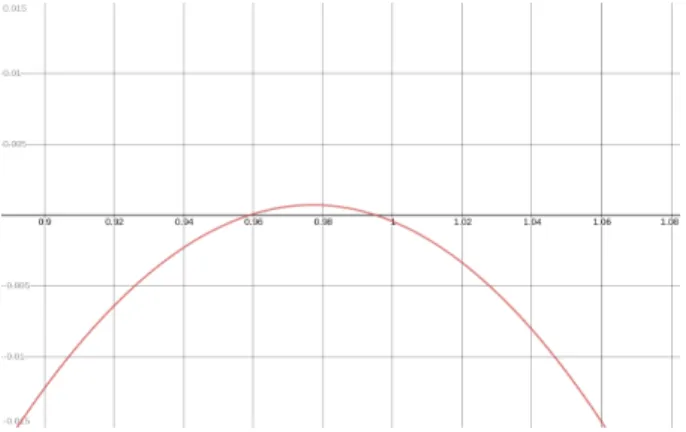
2 and, in particular, it guarantees that if the latter inequality is satisfied then 0 is in fact an interior point of I(p0). In the continuous case, an easy numerical computation gives the sufficient condition cT ≤ 6.318, slightly better than the bound cT ≤ 2π deduced from [10]
(see Figure 1). For arbitraryT, numerical experiments show that 0∈ I(p0)◦ forcT ≤4.19, as shown in Figure 2.
Figure 4.1: Graph ofψforT=RwithcT =6.318
Figure 4.2: Graph ofψfork(T) = T2 andcT =4.19
Remark 4.5. An estimation of the constantk(T)could be obtained analogously to the continu- ous case as shown for example in [13]. Let{en}n∈Z⊂CT be an orthonormal basis ofL2(0,T)T
withe0 ≡ √1
T andEnbe a primitive ofensuch thatEn=0. Writing x∆= ∑n6=0anen, it follows that
kx−xk∞=
∑
n6=0
anEn
≤ kx∆kL2
r
∑
n6=0
kEnk2∞ ≤ kx∆k∞rT
∑
n6=0
kEnk2∞. WhenT=R, taking the usual Fourier basis one has thatkEnk∞ =
√T
2πn and the valuek(R)≤
T 2√
3 is obtained from the well known equality∑n∈Nn12 = π62.
Remark 4.6. As mentioned in the introduction, Theorem 4.1 allows to compute an inferior bound for the length of the solvability interval which does not depend on p0, provided that T is small enough. In some obvious cases, inferior bounds are obtained for arbitrary T: for example, ifkp0k∞ < bthen [−ε,ε] ⊂ I(p0)for ε= b− kp0k∞. This is readily verified taking α= π2 and β= 3π2 as lower and upper solutions.
Acknowledgements
This research was partially supported by projects PIP 11220130100006CO CONICET and UBA- CyT 20020160100002BA.
References
[1] P. Amster, M. P. Kuna, D. P. Santos, Multiple solutions of boundary value problems on time scales for a ϕ-Laplacian operator, Opuscula Math. 40(2020), No. 4, 405–425. https:
//doi.org/10.7494/OpMath.2020.40.4.405
[2] P. Amster, M. P. Kuna, D. P. Santos, Existence and multiplicity of periodic solutions for dynamic equations with delay and singular ϕ-Laplacian of relativistic type, submitted.
[3] C. Bereanu, P. Jebelean, J. Mawhin, Periodic solutions of pendulum-like perturbations of singular and boundedφ-Laplacians,J. Dynam. Differential Equations22(2010), 463–471.
https://doi.org/10.1007/s10884-010-9172-3
[4] C. Bereanu, J. Mawhin, Existence and multiplicity results for some nonlinear problems with singular ϕ-Laplacian,J. Differential Equations243(2007), 536–557. https://doi.org/
10.1016/j.jde.2007.05.014
[5] C. Bereanu, P. J. Torres, Existence of at least two periodic solutions of the forced rel- ativistic pendulum, Proc. Amer. Math. Soc. 140(2012), 2713–2719. https://doi.org/10.
1090/S0002-9939-2011-11101-8
[6] M. Bohner, A. Peterson, Dynamic equations on time scales, Birkhäuser Boston, Mas- sachusetts, 2001.https://doi.org/10.1007/978-1-4612-0201-1
[7] M. Bohner, A. Peterson,Advances in dynamic equations on time scales, Birkhäuser Boston, Massachusetts, 2003.https://doi.org/10.1007/978-0-8176-8230-9
[8] H. Brezis, J. Mawhin, Periodic solutions of the forced relativistic pendulum, Differential Integral Equations23(2010), No. 9, 801–810.https://doi.org/10.1063/1.5129377
[9] A. Castro, Periodic solutions of the forced pendulum equation, in: Differential equa- tions (Proc. Eighth Fall Conf., Oklahoma State Univ., Stillwater, Okla., 1979), Academic Press, New York–London–Toronto, Ont., 1980, pp. 149–160. https://doi.org/10.1016/
B978-0-12-045550-8.50017-7
[10] J. A. Cid, On the existence of periodic oscillations for pendulum-type equations, Adv.
Nonlinear Anal10(2021), 121–130.https://doi.org/10.1515/anona-2020-0222
[11] G. Fournier, J. Mawhin, On periodic solutions of forced pendulum-like equations, J.
Differential Equations60(1985), No. 3, 381–395.https://doi.org/10.1016/0022-0396(85) 90131-7
[12] S. Hilger,Ein Maßkettenkalkül mit Anwendung auf Zentrumsmannigfaltigkeiten(in German), PhD thesis, Universität Würzburg, 1988.
[13] J. Mawhin, Degré topologique et solutions périodiques des systèmes différentiels non linéaires (in French),Bull. Sot. Roy. Sci. Liège38(1969), 308–398.MR594965
[14] J. Mawhin, Periodic solutions of the forced pendulum: classical vs relativistic, Matem- atiche (Catania)65(2010), No. 2, 97–107.https://doi.org/10.4418/2010.65.2.11
[15] J. Mawhin, Global results for the forced pendulum equation, in: Handbook of differ- ential equations: Ordinary differential equations 1, Elsevier/North-Holland, Amsterdam, 2004, pp. 533–589, Elsevier/North-Holland, Amsterdam. https://doi.org/10.1016/
S1874-5725(00)80008-5
[16] J. Mawhin,Topological degree methods in nonlinear boundary value problems, CBMS Regional Conference Series in Mathematics, Vol. 40, American Math. Soc., Providence RI, 1979.
MR525202
[17] K. Prasad, P. Murali, Heteroclinic solutions of singular Φ-Laplacian boundary value problems on infinite time scales, Electron. J. Qual. Theory Differ. Equ. 2012, No. 86, 1–9.
https://doi.org/10.14232/ejqtde.2012.1.86;MR2991442
[18] P. Torres, Periodic oscillations of the relativistic pendulum with friction, Phys. Lett. A.
372(2008), No. 42, 6386–6387.https://doi.org/10.1016/j.physleta.2008.08.060 [19] P. Torres, Nondegeneracy of the periodically forced Liénard differential equation with
φ-Laplacian, Commun. Contemp. Math. 13(2011), No. 2, 283–292. https://doi.org/10.
1142/S0219199711004208