University of Pannonia
Doctoral School of Information Science and Technology
Parameter estimation and robustness analysis of
quantum information systems
PhD thesis by
Gábor Balló
Supervisor:
Dr. Katalin Hangos
March 2, 2014 DOI: 10.18136/PE.2014.546
Parameter estimation and robustness analysis of quantum information systems
Értekezés doktori (PhD) fokozat elnyerése érdekében Írta:
Balló Gábor
Készült a Pannon Egyetem Informatikai Tudományok Doktori Iskolája keretében
Témavezető: Dr. Hangos Katalin
Elfogadásra javaslom (igen / nem) . . . . (aláírás)
A jelölt a doktori szigorlaton 100%-ot ért el.
Az értekezést bírálóként elfogadásra javaslom:
Bíráló neve: . . . igen / nem . . . . (aláírás)
Bíráló neve: . . . igen / nem . . . . (aláírás)
A jelölt az értekezés nyilvános vitáján . . . %-ot ért el.
Veszprém, . . . . a Bíráló Bizottság elnöke
A doktori (PhD) oklevél minősítése . . . .
. . . . az EDT elnöke
Abstract
Quantum information systems have different determining factors of their performance. In particular, in the field of quantum error correc- tion the accurate knowledge of the models of quantum physical pro- cesses, the so-called quantum channels is required. It follows that the ability to accurately identify the channels, together with the precise characterization of error correction robustness properties against the channel uncertainty is essential.
Therefore, the robustness of quantum error correction operations against completely unstructured type of channel uncertainties is first investigated in this thesis. We find that a channel-adapted optimal error correction operation does not only give the best possible channel fidelity but it is more robust against channel perturbations than any other error correction operation. Our results are valid for Pauli chan- nels and stabilizer codes. Numerical results indicate that very similar conclusions can be drawn also in the general case.
In addition, a method of parameter estimation is proposed for quantum channels of which we have a priori structural information.
In the case of channels with the Pauli channel structure, a special parametrization turns the parameter estimation problem into a con- vex optimization problem.
Furthermore, a novel experiment design method for the parameter estimation of Pauli channels is developed both for the cases of known and unknown channel structure. For qubit channels in the former case, this leads to an optimal setting that includes pure input states and projective measurements directed towards the channel directions. For qubit Pauli channels with unknown structure, an iterative method of estimating the channel directions is proposed, together with the study and comparison of an adaptive estimation procedure with simple non- adaptive methods.
i
Kivonat
A kvantum információs rendszerek teljesítményének különféle meg- határozó tényezői vannak. Különönen a kvantum hibajavítás terüle- tén szükséges a kvantumfizikai folyamatok modelljeinek, az úgyneve- zett kvantumcsatornáknak a pontos ismerete. Ebből következik, hogy a csatornák pontos identifikációjának képessége, valamint a hibajaví- tás csatornabizonytalansággal szembeni robusztussági tulajdonságai- nak precíz jellemzése alapvető.
Tehát ebben a disszertációban elsőként a kvantum hibajavító ope- rációk teljesen strukturálatlan típusú csatornabizonytalansággal szem- beni robusztussága kerül vizsgálatra. Azt találjuk, hogy egy csator- naadaptív optimális hibajavító operáció nem csak a lehető legjobb csatornafidelity-t adja, de robusztusabb is a csatornaperturbációkkal szemben, mint bármely más hibajavító operáció. Eredményeink Pauli csatornákra és stabilizátor kódokra érvényesek. Numerikus eredmé- nyek alapján nagyon hasonló következtetések vonhatók le az általános esetben is.
Továbbá egy paraméterbecslő módszert javasolunk olyan kvantum- csatornákhoz, melyek struktúrájáról a priori információnk van. A Pauli struktúrával rendelkező csatornák esetében egy speciális paraméterezés konvex optimalizációs problémává alakítja a paraméterbecslési felada- tot.
Ezenkívül egy újfajta kísérlettervezési módszert fejlesztünk ki a Pauli csatornák paraméterbecsléséhez, ismert és ismeretlen csatorna- struktúra esetére is. Az előbbi esetben kubit csatornákra egy olyan optimális elrendezést kapunk, melyben tiszta bemenő állapotok és pro- jektív mérések állnak a csatornairányok mentén. Ismeretlen struktú- rájú kubit Pauli csatornákra egy iteratív módszert javasolunk a csa- tornairányok becslésére, valamint tanulmányozunk egy adaptív becslő eljárást, melyet összevetünk egyszerű nemadaptív módszerekkel.
Zusammenfassung
Quantum Informationssysteme haben unterschiedliche Faktoren in ihrer Leistung. Insbesondere im Bereich der Quanten-Fehlerkorrektur sind die genauen Kenntnisse von den Modellen des quantenphysikalis- chen Prozesses, die sogenannten Quantenkanäle erforderlich. Daraus folgt, dass die Fähigkeit die Kanäle genau zu identifizieren, zusammen mit der genauen Charakterisierung der Robustheitseigenschaften von der Fehlerkorrektur gegen den Kanal Unsicherheit wesentlich ist.
Daher wird die Robustheit der Quanten-Fehlerkorrektions Opera- tionen gegen völlig unstrukturierte Kanal Unsicherheits Typen erstens in dieser Arbeit untersucht. Wir finden, dass eine optimale Kanal- adaptive Fehlerkorrektur Operation nicht nur den bestmöglichen Kanal Fidelity ergibt, aber es ist auch robuster gegen Kanal Störungen als jede andere Fehlerkorrektur Operation. Unsere Ergebnisse gelten für Pauli Kanäle und Stabilisator Codes. Numerische Ergebnisse zeigen, dass sehr ähnlichen Schlussfolgerungen auch im allgemeinen Fall gezo- gen werden können.
Darüber hinaus wird eine Methode zur Parameterschätzung für Quanten-Kanäle, mit a priori Strukturinformationen vorgeschlagen. Im Falle von Kanälen mit dem Pauli Kanalstruktur wird ein spezielles Parametrisierung das Parameterschätzproblem in eine konvexe Opti- mierungsproblem umwandeln.
Zudem wird ein neuartiges Versuchsplanungs-Methode für die Pa- rameterschätzung von Pauli Kanäle sowohl für die Fälle von bekannten und unbekannten Kanal-Strukturen entwickelt. Für Qubit Kanäle führt dies zu einer optimalen Einstellung, die reine Eingangs-zustände und Projektiv-messungen nach Kanal Richtung gerichtet beinhaltet. Für Qubit Pauli Kanäle mit unbekannter Struktur wird eine iterative Meth- ode zur Schätzung der Kanal Richtungen vorgeschlagen, zusammen mit der Untersuchung und Vergleich eines adaptiven Schätzverfahren mit einfachen, nicht-adaptiven Methoden.
iii
Acknowledgement
I am grateful to Dr. Katalin Hangos, my supervisor, for her guidance and support during my PhD studies. Her advices helped me to learn the practice of scientific research.
I would also like to thank Dr. Péter Gurin, the coauthor of the first part of my thesis, for the joint work and inspiration during the early years of my research.
I must also thank Dr. Dénes Petz, László Ruppert, and Dr. Attila Magyar for their advices on my work.
I thank Róbert Galambos for the discussions about science, about being a PhD student, and for the help in running long simulations.
Big thanks goes also to Veronika Baráth, my girlfriend, for her love, and patience during times of hard work on research and publications.
Finally, I am also grateful to my parents for the strong and constant support they gave me during my student years.
Financial support
Financial support was provided by the Hungarian State and the European Union under the TAMOP-4.2.2.A-11/1/ KONV-2012-0072.
v
Contents
1 Introduction 2
1.1 Background and motivation . . . 2
1.2 Aims of the thesis . . . 3
1.3 Structure of the thesis . . . 4
1.4 Notations . . . 5
2 Basic notions 7 2.1 Postulates of quantum mechanics . . . 7
2.1.1 States of quantum systems . . . 7
2.1.2 Time evolution . . . 11
2.1.3 Quantum measurements . . . 12
2.1.4 Composite systems . . . 13
2.2 Quantum channels . . . 14
2.2.1 The Kraus representation . . . 15
2.2.2 The Choi matrix . . . 16
2.2.3 Channels on a qubit . . . 18
2.3 Pauli channels . . . 18
2.3.1 Group theoretic definition on qubits . . . 18
2.3.2 Definition using matrix algebras . . . 18
2.3.3 Qubit Pauli channel . . . 19
2.4 Measures in quantum information . . . 21
2.4.1 Distance of states . . . 21
2.4.2 Channel performance . . . 21
I Quantum error correction 23
3 Theory of quantum error corretion 24 3.1 Standard QEC . . . 243.1.1 Basic theory . . . 24
3.1.2 Pauli errors on stabilizer codes . . . 27
3.2 Optimal QEC . . . 28
3.2.1 Pauli case . . . 29
CONTENTS
4 Robustness of quantum error correction 31
4.1 Robustness in the context of QEC . . . 31
4.1.1 Perturbation of quantum channels . . . 32
4.1.2 Efficiency of correction on the mixed channel . . . 33
4.1.3 Robustness domains . . . 33
4.2 Robustness in the Pauli channel case . . . 34
4.2.1 Results for the case of single syndrome subspace . . . 35
4.2.2 Results for the general case . . . 37
4.2.3 Geometric picture of Pauli robustness domains . . . 38
4.3 Case studies for non-Pauli channels . . . 41
4.3.1 Pauli channel with non-Pauli perturbation . . . 42
4.3.2 Non-Pauli channel with Pauli perturbation . . . 43
4.3.3 Mixing of non-Pauli channels . . . 44
4.4 Summary . . . 45
II Quantum process tomography and experiment de- sign 47
5 Theory of quantum process tomography 48 5.1 Quantum tomography . . . 485.1.1 Quantum tomography as an identification problem . . . 48
5.1.2 Quantum state tomography . . . 49
5.2 Quantum process tomography . . . 49
5.2.1 Statistical model . . . 50
5.2.2 Experimental data collection . . . 50
5.2.3 Estimation procedure . . . 50
5.3 Experiment design . . . 52
5.3.1 Fisher information . . . 52
6 Parameter estimation for Pauli channels 54 6.1 Parameter estimation of quantum channels . . . 54
6.1.1 Affine approximation . . . 55
6.1.2 Convex constraints . . . 55
6.1.3 Determining the model parameters . . . 56
6.1.4 General example to parameter estimation . . . 57
6.2 Estimation of Pauli channels . . . 58
6.2.1 Qubit Pauli channel . . . 58
6.2.2 Pauli channels for prime-level systems . . . 58
6.3 Case studies . . . 60
6.3.1 Tomography settings . . . 60
6.3.2 Experiment configurations . . . 61
6.3.3 Qubit Pauli channel examples . . . 63
6.3.4 3-level Pauli channel example . . . 66
6.4 Summary . . . 67 vii
CONTENTS
7 Experiment design for Pauli channels with known structure 68
7.1 Problem statement of experiment design . . . 68
7.1.1 The optimization problem . . . 69
7.2 Experiment design for Pauli channels . . . 70
7.2.1 Optimal configuration for qubit Pauli channels . . . 70
7.2.2 Generalization to higher level Pauli channels . . . 72
7.2.3 Analytical solution of parameter estimation . . . 76
7.3 Case studies . . . 77
7.3.1 Optimal estimation of qubit Pauli channel . . . 77
7.3.2 Optimal estimation of 3-level Pauli channel . . . 79
7.4 Summary . . . 80
8 Identification of a Pauli channel with unknown structure 82 8.1 Problem statement . . . 82
8.2 Channel direction estimation . . . 83
8.2.1 Estimation algorithm for channel directions . . . 84
8.2.2 A simple numerical example . . . 86
8.3 Adaptive channel estimation . . . 87
8.3.1 Adaptive estimation algorithm for quantum channels . . 88
8.3.2 Qubit Pauli case . . . 89
8.3.3 Non-adaptive methods . . . 90
8.3.4 Case studies . . . 90
8.4 Summary . . . 92
9 Conclusions 94 9.1 New results . . . 94
9.2 Further work . . . 96
9.3 Publications . . . 96
A Basic notions in mathematics and information theory 100 A.1 Basics of Hilbert spaces . . . 100
A.1.1 The Hilbert space . . . 100
A.1.2 Linear operators on Hilbert spaces . . . 100
A.1.3 Dual space and tensor product . . . 102
A.2 Convex optimization . . . 102
A.2.1 Convex functions . . . 102
A.2.2 Convex optimization . . . 103
A.2.3 The semidefinite programming problem . . . 104
A.3 Group theory . . . 105
A.3.1 General concepts . . . 105
A.3.2 The stabilizer formalism . . . 106
A.4 Matrix algebras . . . 108
A.5 Some more notions and results from QEC . . . 110
A.5.1 Example quantum channels . . . 110
A.5.2 Stabilizer codes . . . 112
CONTENTS
A.5.3 The quantum Hamming-bound . . . 113
A.5.4 The five-qubit code . . . 114
A.5.5 Comparison of standard and optimal QEC . . . 115
A.6 Numerical simulation tools . . . 117
B Supplementary material on channel param. estimation and exp. design 118 B.1 Further examples for Pauli channel estimation . . . 118
B.1.1 Qubit Pauli channel . . . 118
B.1.2 Pauli channel for a 3-level quantum system . . . 118
ix
Chapter 1 Introduction
Atoms on a small scale behave like nothing on a large scale, for they satisfy the laws of quantum mechanics. So, as we go down and fiddle around with the atoms down there, we are working with different laws, and we can expect to do different things.
– R. P. Feynman
According to Feynman, quantum mechanics offers special possibilities, how- ever, it also puts special obstacles in front of these possibilities. For instance, the building of quantum computers that can be used to solve realistic, large scale problems – including the breaking of cryptographic codes and the simula- tion of complex quantum systems – has two main difficulties from the theoret- ical point of view. The first is decoherence, in other words the unwanted but unavoidable coupling of quantum systems with their environment. This noise effect can alter or even completely destroy the information content of the sys- tem, causing errors in the calculation. The other main obstacle is the inability to fully manipulate and extract full information from physical systems, i.e., the control and estimation of quantum states and processes. This is a hard problem, because in quantum mechanics one has to face the difficulty of the treatment of measurements. Namely, that no measurement can be carried out on a quantum system without substantially disturbing the state of the system itself.
1.1 Background and motivation
A common element of the above introduced problems is the quantum chan- nel, i.e., the general model of physical processes transforming quantum states to quantum states. Whether we would like to do quantum information pro- cessing or solve system- and control theoretic problems, the characterization of quantum channels, i.e., the modeling of quantum mechanical processes be- comes essential.
Modeling is an important field in classical system- and control theory [1, 2].
Mathematical models are in general simplifictions of the physical reality, which
1.2. Aims of the thesis
implies that all mathematical models of a physical system suffer from inaccu- racies. These can result from non-exact measurements or from the inability to capture all involved physical phenomena or just from the requirement to obtain a simple model. The quality of a nominal model depends on how closely its be- haviour matches that of the true system. In engineering context this mismatch between the nominal model and the real system is called uncertainty [3], refer- ring not to the uncertain nature of the physical system, but to our incomplete knowledge. The degree of uncertainty can vary from incomplete knowledge about the model structure to uncertainty only in certain parameters.
The design of more accurate nominal models is not necessarily satisfactory in practice, mostly because the real system may not even be in the set of pos- sible nominal models. Thus to have sufficient information about the usability and accuracy of the identified model, robustness analysis of some application specific property against the model uncertainty is also required [4, 3]. Robust- ness in general means the ability to resist change in certain conditions without adaptation. It means that robustness can only be analyzed after the precise characterization of these conditions.
The same problem arises in connection with the processing and control of quantum systems. The complexity of the environment does not allow us to take interactions between the system and its environment into account with perfect accuracy. Thus the quantum channel, too, will always remain just a model, which though describes reality more or less precisely, but we can not assume that it is fully accurate.
It is clear that each quantum information theoretic application has a spe- cific threshold of performance. For instance, the error correction of quantum systems requires accurate models of the channels representing noise processes.
This implies that accurate identification of quantum channels together with the study of the constraints on their uncertainty under which robustness prop- erties hold are of essential importance.
1.2 Aims of the thesis
One of the central problems of quantum information processing is to find suitable error correcting procedures [5, 6]. Therefore, the development of the theory of quantum error correction (QEC) was a very important step, giving the possibility for quantum information theory to become a potentially appli- cable science from an only theoretically interesting field. Nowadays, there are two main approaches; the standard quantum error correcting method tries to adapt the techniques of classical information theory, while the optimization approach can be used – assuming some exact noise model – to find the best error correcting method.
In this thesis, one of our aims is to perform robustness analysis on the con- ventional and optimization based channel specific error correction procedures, assuming uncertainty in the channel model. At first sight, we could think that the conventional QEC – which makes very slight assumptions about the properties of the channel – is more insensitive to the uncertainties than an 3
1. Introduction
error correction optimized for a specific channel. On the other hand, we can also think that if a solution is optimal, then in general, in case of a very small alteration of the conditions it decays only in second order, so it is robust in some measure. These questions apparently have greater significance when the channel is of general type, but because of the simplicity of the handling of Pauli channels, here we concentrate mainly on this specific case.
Another undoubtedly fundamental problem of quantum information theory is the task of the identification of quantum processes, commonly known as quantum process tomography (QPT) [7]. It has considerable relevance not only in quantum computers, but also in the field of quantum communication and cryptography. For example, quantum communication channels usually rely on a priori knowledge of the channel properties. This shows that the performance of quantum information theoretic applications can depend greatly on the accuracy of the estimated channel models.
Thus our second aim is to develop identification methods achieving high accuracy with favorable computational properties. Our convex optimization based approach uses the fact that often we have a priori knowledge of quantum processes, which can be used to reduce the level of uncertainty in the model and arrive at a parameter estimation problem significantly easier to solve with a predefined accuracy.
The problem of classical system identification is related to experiment de- sign, the general aim of which is to determine experimental conditions that result in good or even optimal identification results. In the case of quantum channel parameter estimation, the design variables are the quantum input to the channel, and the measurements to be applied on the resulting quantum output system. These are called the experiment configuration, together with the number of measurements to be performed in the different experiment con- figurations if one has a few of them.
Therefore, our third aim is to extend our results on parameter estimation, and find optimal experiment configurations for the class of Pauli channels having various levels of uncertainty present in the model.
1.3 Structure of the thesis
The rest of the thesis is organized as follows. The introduction is followed by Chapter 2, which describes basic notions about quantum systems and quantum channels.
Part I treats the topic of quantum error correction. In Chapter 3 the basic theory of quantum error correcting methods is introduced. Then Chapter 4 presents our results on the robustness analysis of quantum error correcting procedures against uncertainties of Pauli and non-pauli channels.
Part II treats the topic of quantum process tomography. Chapter 5 gives an introduction on channel identification and the related experiment design problem. Then Chapter 6 presents our results on the convex optimization- based channel parameter estimation of Pauli channels with known structure.
Chapter 7 presents our proposed experiment design method for the estimation
1.4. Notations
of Pauli channels with known channel structure. Finally, in Chapter 8 our two methods for the estimation of Pauli channels with unknown structure is presented.
Lastly, in Chapter 9 the conclusions are drawn in the form of thesis state- ments, the possible future research directions are discussed and the publication list of the author is presented.
Appendix A describes all necessary concepts needed by the main thesis chapters which are assumed beyond the level of an information technology master degree. Appendix B presents additional examples and simulation re- sults complementing those of Chapter 6.
Throughout the thesis, our main results are phrased in the form of state- ments, while used known results are phrased as theorems.
1.4 Notations
Here in Table 1.1 we set a few notational conventions which we will use throughout the thesis. If the meaning of some of these symbols were different in exceptional cases, it will be apparent from the context.
5
1. Introduction
Symbol Meaning H Hilbert space
B(H) set of (bounded) linear operators acting on H
B(H1,H2) set of (bounded) linear operators mapping H1 to H2
V vector space
d level of quantum system
|.i,h.| state vector, dual of state vector ρ density matrix
ρms, ρcs message, codeword
V matrix whose columns form a MUB S qubit Pauli channel affine representation λ Pauli channel depolarizing parameters σx, σy, σz Pauli matrices
X, Y, Z Pauli matrices
Xi, Yi, Zi Pauli matrices acting on the ith qubit X,¯ Y ,¯ Z¯ logical Pauli matrices
|eii,|−eii eigenvectors of σi
|vii,|−vii eigenvectors of vi ·~σ
1 identity matrix θ Bloch vector
C,CS quantum code, stabilizer code E quantum noise channel
R recovery operation XE choi matrix ofE
I identity map
∗ Hermitian adjoint
⋆ denotes optimality
∝ denotes proportionality
∇p gradient with respect to p
∂pi partial derivative with respect topi
VLS least squares objective function
diag(a) matrix with vectora in its main diagonal
diag−1(A) vector obtained by taking out the main diagonal of matrix A
Table 1.1. Notations used in the thesis.
Chapter 2
Basic notions
Here we give a short description of the basic notions of finite dimensional quantum mechanical systems with emphasis on the concepts needed to un- derstand the main chapters. The concepts discussed here can be found in [5, 8]. The mathematical preliminaries needed for the basic notions are briefly summarized in appendix A.
In section 2.1 the postulates of quantum mechanics are presented. Section 2.2 gives a detailed discussion on quantum channels in general. This is followed by section 2.3 on Pauli channels. Then, in section 2.4 several metrics used in quantum information are presented.
2.1 Postulates of quantum mechanics
Quantum mechanics is a mathematical framework used to develop physical theories. It does not give us any laws of physics or tell us any facts about specific physical systems, rather it can be used as a tool for formally describing these laws.
In the next few sections we give an introduction on the basic postulates of quantum mechanics. These postulates provide a connection between the physical world and the mathematical formalism of quantum mechanics. The derivation of the postulates was historically a long process of trial and error, understanding their motivation and meaning can lead to philosophical ques- tions. In this chapter we restrict ourselves only to an application oriented discussion.
2.1.1 States of quantum systems
Two commonly used representations of finite dimensional quantum systems will be presented here, the latter being the most general.
Postulate 1. The state space of any isolated physical system is a complex Hilbert space H. The system can be completely described either by the state vector in H or by the density matrix acting on H.
For finite dimensional quantum systems the dimension d ofH is finite and d is also the dimension (level number) of the quantum system.
7
2. Basic notions
Pure states
A quantum state providing maximal knowledge about the quantum system is said to be a pure state. A pure state is most commonly represented as a normalized state vector |ψi ∈ H. The symbol |ψi is the so-called Dirac “ket”
notation of vectors. By the Dirac notation, the scalar product of two vectors is denoted by hϕ|ψi, where the hϕ| “bra” vector is the natural pair of |ϕi in the dual space.
The linear structure of H implies the superposition principle, namely that the normalized linear combination of two state vectors is also a possible quan- tum state. We can thus write any quantum state |ψi ∈ H as a normalized linear combination P
iαi|ii (αi ∈ C) of an arbitrary orthonormal basis {|ii}
of H with the normalization conditionP
i|αi|2 = 1.
Note that the description of the physical state by a state vector is unique only apart from global phase, i.e., |ψi and eiθ|ψi describe the same physical state. In case of two superposed states however, the phase difference between the corresponding state vectors is relevant.
Mixed states
If the state is not pure, then it is said to be amixed state. A mixed state is represented as a positive semidefinite matrixρ with unit trace, called density matrix:
ρ≥0, Tr(ρ) = 1
Such states are mixtures of pure states taken from the ensemble {pi,|ψii}di=1. This means that the system may be in the pure state|ψii with probabilitypi. Because of this uncertainty, a mixed state does not provide maximal knowledge about the system. The density matrix corresponding to the ensemble is ρ = P
ipi|ψiihψi|.1 It follows that the density matrix of pure states are rank-1 orthogonal projections ρ=|ψihψ|.
The level of mixedness can be measured with the quantity Tr(ρ2) called purity. The value goes from 1 indicating a pure state to 1d indicating the completely mixed stateρ= 1d1 corresponding to the ensemble{1d,|ψii}di=1 for ad level system.
Physical content of the density matrix
Regarding the physical content of a density matrix [9], let ρ be the pure state|ψihψ|. In a given basis|ii, the diagonal elementshi|ρ|iiare referred to as populations, these give the weight|αi|2of the basis state|iiin the superposition
|ψi = P
iαi|ii.2 The off-diagonal elements hi|ρ|ji (with i 6= j) are called coherences, they give information about the relative phase between components of the superposition |ψi. For an ensemble {pk,|ψki}dk=1, these relative phases
1This correspondence is not one-to-one, there is a unitary freedom in the ensembles giving the same density matrix.
2Precisely, these are the probabilities|hi|ψi|2of jumping into the state|iiafter measuring in the basis{|ii}(see later in section 2.1.3).
2.1. Postulates of quantum mechanics
may be different for different pure states |ψki, thus in a mixed density matrix the coherences may get averaged out.
The qubit
The most basic data unit of quantum information theory is the two-state (two-level) quantum system. This is called “quantum bit”, or qubit for short.3 The possible pure states of a qubit are the elements of the two dimensional Hilbert space. After choosing e.g. the orthonormal basis {|0i,|1i} – the so- called computational basis – the states can be written as |ψi =α0|0i+α1|1i, where |α0|2 +|α1|2 = 1. Thus in contrast to the classical bit, which can only be 0 or 1, the qubit can also take the arbitrary complex superposition of the states |0i and |1i.
Let |ψ0i =α0|0i+α1|1i and |ψ1i=β0|0i+β1|1i be pure states. Then all (including mixed) states of a qubit corresponding to the ensemble{pi,|ψii}i=1,2 can be written as the density matrix:
ρ= X1
k=0
pk|ψkihψk|= X
i,j∈{0,1}
ci,j|iihj|, ci,j =p0αiα∗j +p1βiβj∗ (2.1)
In effect, the rank-1 matrices {|iihj|} (i, j ∈ {0,1}) form the computational basis in the complex Hilbert space of all 2×2 matrices.
The Bloch picture
The density matrix of a qubit can be described in any basis similarly to (2.1), however, the most convenient basis is the Pauli basis. It consists of the identity matrix 1 (also denoted σ0 for convenience) and the three Pauli matrices σx (σ1),σy (σ2), andσz (σ3), or simply X,Y, and Z. Their matrices in the computational basis are:
σx=
0 1 1 0
, σy =
0 −i i 0
, σz=
1 0 0 −1
. (2.2)
The Pauli matrices are self-adjoint and they obey the commutation relations σaσb = δab1 + iεabcσc where εabc is the Levi-Civita symbol.4 The symbol ~σ commonly denotes the formal vector [σx, σy, σz]. A formal dot product with v∈R3 is thenv·~σ := P3
i=1viσi.
The convenience in using the basis{1, σx, σy, σz}arises from the fact that it forms an orthogonal basis (with respect to the Hilbert–Schmidt inner product (A.1)) also in the real Hilbert space of 2×2 Hermitian matrices. The qubit
3Considering its specific physical realization, the qubit can be the spin of any half-integer spin particle (for example the spin of an electron), or the two different polarization states of a photon.
4If(a, b, c)is an even permutation of(x, y, z), then εabc = 1, in case of odd permutation εabc=−1, elseεabc= 0.
9
2. Basic notions
density matrices can thus be written as ρ= 1
2 1+ X3
i=1
θiσi
!
= 1 2
1 +θ3 θ1−iθ2
θ1+ iθ2 1−θ3
, (2.3)
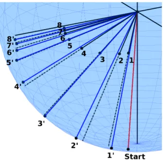
where the numbersθi = Tr(ρσi)form a three-dimensional vector θ, commonly called Bloch vector. The hermiticity and normalization of the density matrix are ensured by this formula. The remaining positivity constraint is expressed using the 2-norm of the Bloch vector askθk2 ≤1. It follows that equation (2.3) gives a unique correspondence between all possible qubit states and points of the unit ball inR3, the so-called Bloch ball, which can be seen in Figure 2.1.
Let |eii and |−eii be the normalized eigenvectors of the Pauli matrix σi
from the expansion
σi =|eiihei| − |−eiih−ei|.
Through the correspondence (2.3), |eii and |−eii are identified with the two unit vectors±ei along the Cartesian axis i.
The Bloch vector picture of qubits allows a convenient distinction of pure and mixed states. The pure (completely polarized) states take place on the surface of the Bloch ball, and the mixed (depolarized) states can be found in the interior, with decreasing purity towards the origin representing the completely mixed (completely depolarized) state.
Mutually unbiased bases
It is well-known that the three bases{|eii,|−eii}3i=1 form a set of mutually unbiased bases (MUB) (see appendix A.4). MUBs can be unitarily transformed
Figure 2.1. It can be seen on the Bloch sphere, that all pure states of a qubit can also be written in|ψ(θ, ϕ)iform.
2.1. Postulates of quantum mechanics
into each other. In the case of qubits, since any orthogonal transformation V = [vx,vy,vz] on R3 is induced by a unitary conjugation with UV on 2×2 complex matrices, the basis vectors{UV|±eii}will be the eigenvectors ofvi·~σ corresponding to the Bloch vectors ±vi. A set of MUB can then be identified with three orthogonal axes in the Bloch ball, and any two-dimensional MUB arises this way. Thus, the general notation |±vii := UV|±eii will be used in the following.
This symmetry of the Bloch ball shows that any MUB {|±vii}3i=1 on qubit systems can be used to describe qubit density matrices as Bloch vectors with respect to the MUB {|±vii}:
ρ= 1 2 1+
X3
i=1
ϑivi·~σ
!
= 1 2 1+
X3
i=1
ϑi(|viihvi| − |−viih−vi|)
!
(2.4)
= 1 2 1−
X3
i=1
ϑi
!
1+ X3
i=1
ϑi|viihvi| ,
where ϑi = Tr(ρvi·~σ) = vTi θ is now a vector component in the basis {vi}3i=1.
2.1.2 Time evolution
Postulate 2. The continuous time evolution of a closed quantum system |ψi is described by the Schrödinger equation
d
dt|ψ(t)i=−i
~H|ψ(t)i , (2.5)
where ~ is the Planck’s constant, and H is a fixed hermitian operator known as the Hamiltonian of the closed system.
If we know the Hamiltonian of a quantum system, then (in principle) we understand its dynamics completely.5 The value of ~ is not important for us, practically it can just be absorbed into H.
The solution of this equation is |ψ(t)i = e−i(t−t0)H|ψ(t0)i, which indicates that the unitary matrixU(t, t0) = e−i(t−t0)H calledtime-evolution operator can be used to easily relate states at different time instants, i.e., to implement discrete time dynamics. It can be proven that any unitary arises in such form, thus the state dynamics governed by (2.5) is also known as unitary evolution.
The property of reversibly relating two quantum states allows us to regard unitaries also asquantum logic gates, and use them to implement analogues of classical reversible logic circuits.6
It must be noted that no such unitaryU exists that could create an indepen- dent copy of an arbitrary quantum state|ψi, i.e., act asU(|ψi⊗|0i) =|ψi⊗|ψi for all |ψi ∈ H. Such U exist only for sets of mutually orthogonal states, so
5In general, figuring out the Hamiltonian is a difficult problem in physics.
6Classical irreversible gates do not have a quantum analogue, because quantum computa- tion is practically done on pure states, and irreversible quantum dynamics does not preserve purity, i.e., it acts as noise (see section 2.2).
11
2. Basic notions
copiers can only be constructed for the elements of a known basis of H. This is the content of the so-calledno-cloning theorem.
The equivalent of equation (2.5) for mixed states is the von Neumann equation dtdρ(t) =−~i[H, ρ(t)], and analogously ρ(t) =U(t, t0)ρ(t0)U(t, t0)∗.
The simplest examples of quantum gates are the Pauli matrices (2.2). The matrix X is known as the quantum not gate or bit-flip suggested by the expression X|0i = |1i. Similarly, Z is called phase-flip because it flips the relative phase: Z(α0|0i+α1|1i) = α0|0i−α1|1i,|α0|2+|α1|2 = 1. Furthermore, asY is proportional with XZ, we call it bit-phase flip.
2.1.3 Quantum measurements
Observing a quantum system, i.e., taking a measurement is a special ex- ample of non-unitary quantum dynamics.
Postulate 3. Quantum measurement procedures are represented by a collection M := {Mm} of self-adjoint positive operators acting on the state space H of the system being measured. The index m identifies each operator Mm with a corresponding outcome event that may occur as a result of the measurement.
This implies that{Mm} has to satisfy the completeness relation P
mMm =1. Such a set of operators are commonly called positive operator-valued measure (POVM).
If the system is in state ρ then the probability distribution of possible out- comes is given byp(m|ρ) = Tr(ρMm). If we get the measurement result m and the measurements are further specified7 such that Mm =Fm∗Fm uniquely, then the state ρ of the system collapses8 into ρm = Fp(mmρF|ρ)m∗.
Thus the main features of quantum measurement are the stochastic out- come and the unavoidable abrupt back-action on the measured system, making the state change discontinuously.
POVMs form a convex set [10]. M = pM1+ (1−p)M2 with 0 ≤ p ≤ 1 means that the distributionpM(.|ρ) can be equivalently obtained as the con- vex combination of pM1(.|ρ) and pM2(.|ρ), i.e., measuring M is the same as randomly choosing between measurements M1 and M2. Formally, the con- vex combination of POVMs is calculated elementwise by treating POVMs as vectors of positive operators (with elements allowed to be the zero operator).
The extremal points of the set of POVMs are called extremal POVMs. Let {|ψα,ii}rank(Mi=1 α) be the set of eigenvectors of POVM element Mα. Then the POVM M = {Mα} is extremal if and only if the operators |ψα,iihψα,j| are linearly independent for allα, i and j.
7In spite of this inconvenience, POVMs are widely used, because in many cases only the measurement statistics are important.
8This means that measurement makes the state ρjump into one of the possible outcome statesρm.
2.1. Postulates of quantum mechanics
Projective measurement
If the positive operators are all orthogonal projections Pm onto pairwise orthogonal subspaces, then we have a special case of measurements, the so- called projective (von Neumann–Lüders) measurement.
This property allows projective measurementsM={Pm}to be represented as a single observable M, a Hermitian operator on the state space H of the system. The correspondence is made using the spectral decomposition M = P
mmPm, i.e., each Pm will be a projector onto the eigenspace of M with eigenvalue m. If the projections are all of the form Pm =|mihm| then we can speak about “measuring in the basis |mi”.
Furthermore, the hermiticity and idempotence of Pm allows us to derive the state after measurement directly; performing a projective measurement collapses the state into one of the eigenvectors (eigenstates) of the measured M observable. It follows that projective measurements – opposed to POVMs – are repeatable in the sense that repeating the same measurement will give the same result with certainty.
It can be proven that POVMs can be realized as projective measurements if we are allowed to compose the system with other quantum systems and to perform unitary dynamics.
Projective measurements are included in the set of extremal POVMs.
Observables for qubits are for example the Pauli matrices.9 Let us have the state |ψi = α0|0i+α1|1i. Measuring in the computational basis corre- sponds to the observable σz =|0ih0| − |1ih1| or to the POVM {|0ih0|,|1ih1|}. Then the state of the qubit after measurement will be |0i with probability Tr(|ψihψ|0ih0|) = |α0|2, and |1i with probability Tr(|ψihψ|1ih1|) = |α1|2. However, if we only know that a measurement has happened, but the result is unknown, then the state of the system can be given as the ensemble of the two possible outcome states, i.e., as the density matrix
ρ=|α|2|0ih0|+|β|2|1ih1| .
In general, every projective measurement on a qubit can be written as a two element POVM. In the Bloch picture these two elements are 12(1±v·~σ)with kvk2 = 1, and they can be used for “measurement along the axis v” in the Bloch ball. After measurement, the state changes either to the Bloch vector v or −v.
2.1.4 Composite systems
Postulate 4. The state space H of a bipartite physical system is the tensor product (see appendix A.1.3) H1 ⊗ H2 of the state spaces H1 and H2 of the component systems. Moreover, if the first system is in state|ψ1iand the second system is in state|ψ2ithen the joint state of the total system is|ψ1i⊗|ψ2i ∈ H.
9Historically, observables correspond to physical quantities. The Pauli matrices can be used to measure spin components, while the Hamiltonian from section 2.1.2 is the observable of energy.
13
2. Basic notions
An arbitrary state of the spaceHcan then be written in the following way:
|ψi=X
i,j
αi,j|ii ⊗ |ji, or in short |ψi=X
i,j
αi,j|iji , (2.6) where|ii and |ji are orthonormal bases for the component Hilbert spaces H1 and H2.
If in (2.6) |ψi = P
iαi|ii ⊗P
jαj|ji = |ψ1i ⊗ |ψ2i with |ψ1i ∈ H1 and
|ψ2i ∈ H2, then |ψi is called a separable state. Otherwise, if the component systems can not be separated, then|ψiis anentangled state. This means that there is a quantum correlation between its component systems.
However, even if|ψiis entangled, we can still associate for example its first subsystem with a state, which provides the correct measurement statistics for measurements affecting only the first subsystem, i.e., measurements having POVM elements of the form Mm ⊗1. It is calculated using the partial trace defined as the unique linear operator Tr1: B(H1⊗ H2) → B(H2) such that Tr1(A1⊗A2) = A2Tr(A1). Then the partial trace of |ψi with respect to the second subsystem is
ρ1 = Tr2(|ψihψ|) = X
i,j,k,l
αi,jα∗k,l|iihk| ⊗Tr(|jihl|) =X
i,j,k
αi,kα∗k,j|iihk| . (2.7) The resultρ1 is called reduced density operator. In terms of reduced densities,
|ψiis entangled if and only if ρ1 (and ρ2) is mixed, indicating that we can not get maximal knowledge of them independently of the other part of|ψi. Thus, any mixed stateρ1 can be obtained as a correlated part of some larger system.
Moreover, assuming that dim(H1) ≤ dim(H2), |ψi is said to be maximally entangled ifρ1 = Tr2(|ψihψ|) = dim(1H
1)1, i.e.,ρ1 is a maximally mixed state.
To find a pure state|ψi for which (2.7) holds with a given mixedρ1 as sub- system is calledpurification of ρ1. This procedure is of course not unique, the system and its environment as a whole can have many states whose subsystem is the same mixed state.
Consider now the two-qubit state |Φ+i= √12(|00i+|11i). This state is an example of entangled state; there are no single qubit states|φ1iand |φ2i such that|Φ+i=|φ1i ⊗ |φ2i. In fact, the partial traces ρ1 = Tr2(|Φ+ihΦ+|) = 121= Tr1(|Φ+ihΦ+|) = ρ2result in mixed states. The resultρ1 =ρ2 = 121also shows that |Φ+i is a two-qubit maximally entangled state.
Operators acting independently on each part of a composite system are also in tensor product form. For example, the tensor product of Pauli matrices can act on multiple qubit systems: (X ⊗Z)(α|0i +β|1i) = αX|0i+βZ|1i = α|1i −β|1i. X⊗Z can also be denoted as X1Z2 meaning that X acts on the first qubit andZ acts on the second.
2.2 Quantum channels
In reality, a quantum system can never be perfectly closed. The interaction with the environment gives rise to more general physical processes causing
2.2. Quantum channels
dynamic change in the state necessarily represented as a density matrix. These processes are thus modeled by quantum channels (or quantum operations) which map density matrices to density matrices.10 In the following, we will present different mathematical representations of channels with their respective properties.
2.2.1 The Kraus representation
One way to arrive at a definition of the quantum channel E is to consider the quantum system together with its environment to be closed. Let ρ be the density matrix of the system with state space H1, and let the environment with state space H2 be in some pure state |ϕ0i.11 Then the unitary evolution of the joint state ρ⊗ |ϕ0ihϕ0| is U(ρ⊗ |ϕ0ihϕ0|)U∗. From this we get the dynamics of the H1 system alone by taking the partial trace with respect to the environment H2. This gives us the first definition of quantum channels:
E(ρ) = Tr2 U(ρ⊗ |ϕ0ihϕ0|)U∗
=X
j
hϕj|U|ϕ0iρhϕ0|U∗|ϕji=X
j
VjρVj∗ (2.8) If{|ii ⊗ |ϕji}is an orthonormal basis ofH1⊗ H2, thenVj :=hϕj|U|ϕ0i: H1 → H1 denotes the operator with matrix elements (hi| ⊗ hϕj|)U(|i′i ⊗ |ϕ0i). This operator element set {Vj} gives the so-called Kraus representation of E. Be- cause of the unitarity of U it also holds that
X
j
Vj∗Vj =1 , (2.9)
which is the completeness relation expressing the trace preserving property of E.12
Knowledge of the operator elements {Vj} makes it possible to describe the dynamics of the systemH1 without needing the attributes of the environment H2 to be taken into account explicitly; all nesessary information is embedded into the operator elements, which only have effect on H1. It follows however, that the set of Kraus operators{Vj}corresponding to a particular channelE is not unique. In fact the choice of basis{|ϕji}is arbitrary in (2.8). This implies a unitary freedom in the operator element set for the channel E: the operators Wi =P
jui,jVj (withui,j ∈Cbeing the elements of a unitary matrix) form an equivalent set of Kraus operators for the channel E.13
Note that if we have a d level quantum system, then at most d2 operator elements are enough to describe any possible quantum channel on the system.
10Channels are also called superoperators, because they map operators to operators.
11The environment could also be mixed, however, considering it pure is not a loss of generality. Moreover, ifdim(H1) =dthen it is sufficient to take dim(H2)to be at most d2.
12Measurements can also be modeled using quantum channels, if we relax the completeness condition (2.9) toP
jVj∗Vj≤1.
13If the two operator element sets do not contain the same number of operators, then we augment the smaller set with zero operators.
15
2. Basic notions
Note also that this channel definition can be generalized to the case of different input and output spaces. In this case, instead of making distinction between system and environment spaces, we speak about two systems; the first starts in stateρ, the second is in state|ϕ0i. We bring them into interaction, then by discarding the first system, i.e., by applying the partial trace on it, we obtain the remaining second system in the output stateE(ρ).
Defining axioms
Quantum channels can also be defined as maps satisfying the following axioms:
• linearity: required by the ensemble interpretation of density matrices,
• positivity andtrace preservation: these ensure that the channel out- come will also be a density matrix,
• complete positivity: this means that the composite channel E ⊗ In acting on the extended space B(H1)⊗ B(Hext) with dim(Hext) =n also has to be a positive map for all n.
Maps with these properties are commonly calledcompletely positive and trace preserving (CPTP) maps.
The following theorem states that the above two definitions of quantum channels are equivalent:
Theorem 2.1. A map E:B(H1)→ B(H2)taking density operators to density operators satisfies the above three axioms if and only if E(ρ) = P
jVjρVj∗ for a set {Vj: H1 → H2} satisfying (2.9).
2.2.2 The Choi matrix
The unitary freedom in the Kraus representation can be circumvented using another possible description of channels, theChoi matrix, which is in essence a matrix representation of the channel E. In fact, E has an infinite number of equivalent Kraus representations, but has only one Choi matrix. It can be defined using the Choi–Jamiołkowski isomorphism [11, 12].
The Choi–Jamiołkowski isomorphism
The Choi–Jamiołkowski isomorphism associates an operator C: H1 → H2
with a vector14 |Cii ∈ H1⊗ H2. Let {|i1i} and {|j2i} be some preferred basis inH1 and H2, and let |Φmaxi=P
i|i1i ⊗ |i1i be the unnormalized maximally entangled state in H1 ⊗ H1. Then the isomorphism is given by the following definition:
|Cii:= (1⊗C)|Φmaxi=X
i
|i1i ⊗C|i1i=X
i,j
|i1i ⊗ hj2|C|i1i|j2i
14The|.ii notation tries to indicate that these vectors represent operators.
2.2. Quantum channels
This is essentially the “stacking” of columns of the matrixCto form the vector
|Cii. This assignment is obviously unique, and it also can be seen that|Φmaxi=
|1ii. The inner product of these vectors inH1⊗H2 is defined in a natural way:
hhA|Bii= X
i
hi1| ⊗ hi1|A∗
! X
j
|j1i ⊗B|j1i
!
= Tr(A∗B) (2.10) what is by definition the Hilbert–Schmidt inner product (A.1) of the two oper- ators. Thus an isomorphism can be made between the operators inB(H1,H2) and the vectors of the space H1⊗ H2.
LetATdenote the transposition in the preferred basis{|i1i}. Then a useful relation follows directly from the above definition:
(A⊗B)|Cii=|BCATii , (2.11) whenever the dimensions of A, B, and C indicate that BCAT is a valid oper- ator.15
Representing quantum channels
Using the fact that the space of maps E: B(H1)→ B(H2) is also a Hilbert space, we can use the Choi–Jamiołkowski isomorphism to associateE with an operator XE ∈ B(H1)⊗ B(H2):
XE := (I ⊗ E) (|ΦmaxihΦmax|) =X
i,j,k
|i1i ⊗Vk|i1i
hj1| ⊗ hj1|Vk∗ where the operators Vk are the Kraus operator elements ofE. Continuing the derivation, two useful formulas can be obtained from this:
XE =X
k
(1⊗Vk)|1iihh1|(1⊗Vk∗) = X
k
|VkiihhVk| (2.12) and
XE =X
i,j
|i1ihj1| ⊗X
k
Vk|i1ihj1|Vk∗ =X
i,j
|i1ihj1| ⊗ E(|i1ihj1|) . (2.13) Actually, the above matrix is a block matrix, its (i, j)th element is E |i1ihj1|
. The complete positivity ofE is equivalent to the positivity ofXE. Further- more, E is trace preserving if and only if Tr
E |i1ihj1|
= Tr |i1ihj1|
=δi,j
which means Tr2(XE) = 1.
The inverse of the map, i.e., theXE → E relation isE(ρ) = Tr1 (ρT⊗1)XE , which comes from (2.13).
Note that the definition of the Choi–Jamiołkowski isomorphism presented here is basis dependent, i.e., depends on the choice of{|i1i}.
The Kraus operator elements |Vkii can be obtained from the Choi matrix by applying a square root factorization. The unitary freedom of such a factor- ization corresponds to the unitary freedom of the Kraus representation.
Note also that the Choi matrix representation shows clearly that the set of quantum channels is convex.
15Another relation not used here follows for C1, C2 ∈ B(H1,H2): Tr1(|C1iihhC2|) = C1C2∗∈ B(H2)
17
2. Basic notions
2.2.3 Channels on a qubit
In the two-level system case, as in section 2.1.1 we have the possibility to expand the density operatorρwith respect to any set of MUB{±|vii}3i=1. The most general channel on a qubit can then be associated with an affine map T: R3 →R3 acting on the Bloch ball [8, 13]:
T(θ) =Sθ+t ,
where θ is the Bloch vector of ρ, t ∈ R3 and S = VΛQVT is a real matrix decomposed into rotation matrices Q and V = [v1,v2,v3] with the latter representing the MUB transformation. Finally, Λ is diagonal with elements λ1, λ2, and λ3.
If V and Q are not important and we are free to set them then simply V = Q = 1, and then we have the map T = Λθ +t corresponding to the standard set of MUB{±|eii}3i=1. This form is generally sufficient for analyzing the properties of the channel.
Example qubit channels used throughout the thesis are described in Ap- pendix A.5.1.
2.3 Pauli channels
A notable wide class of quantum channels are the Pauli channels.
2.3.1 Group theoretic definition on qubits
Pauli channels can be defined using the Pauli group defined in appendix A.3.1. If a channel has a set of operator elements, which contains scaled elements of the Pauli group, i.e., {Vi = √aigi} where ai ≥ 0 and gi ∈ Pn, then we call it an n-qubit Pauli channel.16 Because of the trace preserving condition of the channel, P
iai = 1 has to hold. Note that (2.8) implies that two operator element sets differing only in factors of ±1or±i give rise to the same Pauli channel.
On a single qubit, the Pauli channel is thus the following:
V0 =√a01, V1 =√a1X, V2 =√a2Y, V3 =√a3Z, ai ≥0, X
i
ai = 1 (2.14)
2.3.2 Definition using matrix algebras
The most general Pauli channel definition for arbitrary level quantum sys- tems is discussed in [14] in a matrix algebraic context (see appendix A.4 for basics).
Let the center of the full matrix algebra Md(C) be ZMd(C) ={c1|c∈ C}, and letAi :Md(C)→ Ai be a trace preserving projection (usually called condi- tional expectation). If the pairwise complementary subalgebrasA1,A2, . . . ,Au
16In order to be Pauli, it is enough for the channel to have at least one such Kraus element set.
2.3. Pauli channels
of Md(C)are given and they linearly span the whole algebra Md(C), then any matrixD ∈Md(C)is the sum of the componentsAi(D)−Tr(D)d 1in the traceless subspaces Ai∩ZM⊥d(C) and the component Tr(D)d 1 in ZMd(C):
D= Xu
i=1
Ai(D)− Tr(D) d 1
+Tr(D) d 1 ,
By definition, the Pauli channel E is depolarizing on each Ai∩ZM⊥d(C), i.e., contracts each component Ai(D)− Tr(D)d 1 with parameterλi, resulting in
E(D) = 1− Xu
i=1
λi
!Tr(D) d 1+
Xu
i=1
λiAi(D)
Trivially, if D is a density matrix and λi = 0 for all i then the result is the completely mixed state 1d1. Conversely if λi = 1 for all i then D remains unchanged.
The channel is trace preserving by construction, and completely positive if and only if the parameters λi satisfy
1 +dλi ≥X
j
λj ≥ − 1
d−1 . (2.15)
This constraint describes a polyhedron bounded by λi ∈[d−−11,1].
In this thesis, we consider only the case when all of the complementary subalgebras are maximal Abelian, and the leveldof quantum systems is prime number. In this case the subalgebras {Ai}d+1i=1 can be obtained as the linear span of d+ 1groups of unitaries (see appendix A.4), and the unitaries can be selected to be generalized Pauli matrices. Through these, the set of subalgebras correspond also to a set of MUB{|φi,ji}d+1i=1, and thus the orthogonal projection Ai can be constructed as
Ai(D) = Xd
j=1
hφi,j|D|φi,ji|φi,jihφi,j| , and the subalgebras can also be given as
Ai = ( d
X
j=1
cj|φi,jihφi,j|
cj ∈C )
.
2.3.3 Qubit Pauli channel
For qubit systems, a standard selection{±|eii}3i=1of MUB can be obtained from the eigenvectors of the Pauli matrices. Then the
Ai ={a|eiihei|+b|−eiih−ei| |a, b∈C} (i= 1,2,3)
19