Karhunen–Lo` eve expansion for a generalization of Wiener bridge

Karhunen–Lo` eve expansion for a generalization of Wiener bridge

M´aty´as Barczy^∗, and Rezs˝o L. Lovas^∗∗

* MTA-SZTE Analysis and Stochastics Research Group, Bolyai Institute, University of Szeged, Aradi v´ertan´uk tere 1, H–6720 Szeged, Hungary

** Institute of Mathematics, University of Debrecen, Pf. 400, H–4002 Debrecen, Hungary.

e–mails: barczy@math.u-szeged.hu (M. Barczy), lovas@science.unideb.hu (R. L. Lovas).

Corresponding author.

Abstract

We derive a Karhunen–Lo`eve expansion of the Gauss process B_t−g(t)R1

0 g⁰(u) dB_u,t∈[0,1], where (Bt)_t∈[0,1] is a standard Wiener process and g : [0,1] → R is a twice continuously differentiable function with g(0) = 0 and R1

0(g⁰(u))²du= 1. This process is an important limit process in the theory of goodness-of-fit tests. We formulate two special cases with the function g(t) =

√ 2

π sin(πt), t∈[0,1], and g(t) =t, t∈[0,1], respectively. The latter one corresponds to the Wiener bridge over [0,1] from 0 to 0.

1 Introduction

In this note we present a new class of Gauss processes, generalizing the Wiener bridge, for which Karhunen–Lo`eve (KL) expansion can be given explicitly. We point out that there are only few Gauss processes for which the KL expansion is explicitly known. To give some examples, we mention the Wiener process (see, e.g., Ash and Gardner [5, Example 1.4.4]), the Ornstein–Uhlenbeck process (see, e.g., Papoulis [24, Problem 12.7] or Corlay and Pag`es [10, Section 5.4 B]), the Wiener bridge (see, e.g., Deheuvels [12, Remark 1.1]), Kac–Kiefer–Wolfowitz process (see, Kac, Kiefer and Wolfowitz [16] and Nazarov and Petrova [23]), weighted Wiener processes and bridges (Deheuvels and Martynov [13]), Jandhyala–MacNeill process (Jandhyala and MacNeill [15, Section 4]), a generalization of Wiener bridge (Pycke [25]), generalized Anderson–Darling process (Pycke [26]), Rodr´ıguez–Viollaz process (Pycke [27]), scaled Wiener bridges or also called α-Wiener bridges (Barczy and Igl´oi [6]), limit processes related to Cram´er–von Mises goodness-of-fit tests for hypotheses that an observed diffusion process has a sign-type trend coefficient (Gassem [14]), detrended Wiener processes (Ai, Li and Liu [3]), additive Wiener processes and bridges (Liu [18]), additive Slepian processes (Liu, Huang and Mao [19]), Spartan spatial random fields (Tsantili and Hristopulos [28]), the demeaned stationary Ornstein–Uhlenbeck process (Ai [2]), and the additive two-sided Brownian motion (Ai and Sun [4]).

We also mention that KL expansions of Gauss processes have found several applications in small deviation theory, for a complete bibliography, see Lifshits [17]. Here we only mention two papers of Nazarov and Nikitin [20], [22].

2010 Mathematics Subject Classifications: 60G15, 60G12, 34B60.

Key words and phrases: Gauss process, Karhunen–Lo`eve expansion, integral operator, Wiener bridge.

M´aty´as Barczy is supported by the J´anos Bolyai Research Scholarship of the Hungarian Academy of Sciences. Rezs˝o L. Lovas was supported by the Hungarian Scientific Research Fund (OTKA) (Grant No.: K-111651).

arXiv:1602.05084v3 [math.PR] 12 Aug 2018

Let Z+, N and R denote the set of non-negative integers, positive integers and real numbers, respectively. For s, t∈R, we will use the notation s∧t:= min{s, t}. Let (B_t)_t∈[0,1] be a standard Wiener process, and let g : [0,1] → R be a twice continuously differentiable function such that g(0) = 0 and R1

0(g⁰(u))²du= 1. Let us introduce the process Y_t:=B_t−g(t)

Z 1 0

g⁰(u) dB_u, t∈[0,1].

(1.1)

The process Y = (Y_t)_t∈[0,1] appears as a limit process related to a goodness-of-fit test, where one has to decide whether an independent and identically distributed sample has a given continuous distribution function depending on some unknown one-dimensional parameter, see, e.g., Darling [11]

or Ben Abdeddaiem [9] (one can choose h(θ, t) :=g⁰(t), t∈[0,1], in formula (1) in [9]). The process Y also appears as a limit process related to another goodness-of-fit test in the case of continuous time observations of a diffusion process with small noise, see Ben Abdeddaiem [9, formula (5)]. One can consider Y as a generalization of the Wiener bridge corresponding to the function g. In the special case g(t) = t, t ∈ [0,1], we have Yt = Bt−tR1

0 1 dBu = Bt−tB1, t ∈ [0,1], i.e., it is a Wiener bridge over [0,1] from 0 to 0. However, in general, Y is not a bridge. Note that Y is a bridge in the sense that P(Y1 =y1) = 1 with some y1 ∈R (i.e., Y takes some constant value at time 1 with probability one) if and only if g(1)∈ {−1,1}, and in this case y1 = 0. Indeed, P(Y1 =y1) = 1 with some y₁ ∈R if and only if D²(Y₁) = 0. Since D²(Y₁) = 1−(g(1))² (see Proposition 1.1), we have P(Y1 = y1) = 1 with some y1 ∈ R if and only if g(1)∈ {−1,1}, as desired. Further, since E(Y1) = 0, in this case we have y1 = 0. In the present paper, we do not intend to study whether the process (Y_t)_t∈[0,1] given by (1.1) can be considered as a bridge in the sense that it can be derived from some appropriate stochastic process (for more information on this procedure, see Barczy and Kern [7]).

We also give a possible formalmotivation for the definition of the process Y. Let us write (1.1) in the form

dY_t= dB_t− Z 1

0

g⁰(u) dB_u

g⁰(t) dt, t∈[0,1], where

R1

0 g⁰(u) dB_u

g⁰(t) can be formallyinterpreted as the orthogonal projection of the derivative of Bt (in notation dBt) onto g⁰ in L², since R1

0(g⁰(u))²du= 1 (it is only a formalone because the derivative of B does not exist). So, from this point of view, the derivative of Y_t (in notation dY_t) isformallythe orthogonal component of dB_t with respect to g⁰ in L², and one can call dY_t as the g⁰-detrendization of dBt.

Further, we point out that if g additionally satisfies g⁰(1) = 0, then the Gauss process (Yt)t∈[0,1]

given in (1.1) coincides in law with one of the Gauss processes introduced in Nazarov [21, formula (1.3)], for more details, see Appendix A. In the spirit of Nazarov [21], one can say that (Y_t)_t∈[0,1] is a perturbation of the Wiener process (Bt)_t∈[0,1] by the function g.

1.1 Proposition. The process (Y_t)_t∈[0,1] is a zero-mean Gauss process with continuous sample paths almost surely and with covariance function R(s, t) := Cov(Y_s, Y_t) =s∧t−g(s)g(t), s, t∈[0,1].

The proof of Proposition 1.1 can be found in Section 2.

The continuity of the covariance function R yields that (Y_t)_t∈[0,1] is L²-continuous, see, e.g., Theorem 1.3.4 in Ash and Gardner [5]. We also have R ∈ L²([0,1]²). So, the integral operator

associated to the kernel function R, i.e., the operator AR:L²([0,1])→L²([0,1]),

(1.2) (AR(φ))(t) :=

Z 1 0

R(t, s)φ(s) ds, t∈[0,1], φ∈L²[0,1],

is of the Hilbert–Schmidt type, thus (Yt)_t∈[0,1] has a Karhunen–Lo`eve (KL) expansion based on [0,1]:

(1.3) Y_t=

∞

X

k=1

pλ_kξ_ke_k(t), t∈[0,1],

where ξ_k, k ∈N, are independent standard normally distributed random variables, λ_k, k ∈N, are the non-zero (and hence positive) eigenvalues of the integral operator AR and ek(t), t∈[0,1], k∈N, are the corresponding normed eigenfunctions, which are pairwise orthogonal in L²([0,1]), see, e.g., Ash and Gardner [5, Theorem 1.4.1]. For completeness, we recall that the integral operator A_R has at most countably many eigenvalues, all non-negative (due to positive semi-definiteness) with 0 as the only possible limit point, and the eigenspaces corresponding to positive eigenvalues are finite dimensional. Observe that (1.3) has infinitely many terms. Indeed, if it had a finite number of terms, i.e., if there were only a finite number of eigenfunctions, sayN, then, by the help of (1.1), we would obtain that the Wiener process (B_t)_t∈[0,1] is concentrated in an at most (N + 1)-dimensional subspace of L²([0,1]), and so even of C([0,1]), with probability one. This results in a contradiction, since the integral operator associated to the covariance function (as a kernel function) of a standard Wiener process has infinitely many eigenvalues and eigenfunctions. We also note that the normed eigenfunctions are unique only up to sign. The series in (1.3) converges in L²(Ω,A,P) to Yt, uniformly on [0,1], i.e.,

sup

t∈[0,1]

E





Yt−

n

X

k=1

pλkξkek(t)

2

→0 asn→ ∞.

Moreover, since R is continuous on [0,1]², the eigenfunctions corresponding to non-zero eigenvalues are also continuous on [0,1],see, e.g. Ash and Gardner [5, p. 38] (this will be important in the proof of Proposition 1.2, too). Since the terms on the right-hand side of (1.3) are independent normally distributed random variables and (Yt)t∈[0,1] has continuous sample paths with probability one, the series converges even uniformly on [0,1] with probability one (see, e.g., Adler [1, Theorem 3.8]).

1.2 Proposition. If λ is a non-zero (and hence positive) eigenvalue of the integral operator A_R and e is an eigenfunction corresponding to it, then

λe⁰⁰(t) =−e(t)−g⁰⁰(t) Z 1

0

g(s)e(s) ds, t∈[0,1], (1.4)

with boundary conditions

e(0) = 0 and λe⁰(1) =−g⁰(1) Z 1

0

g(s)e(s) ds.

(1.5)

Conversely, if λ and e(t), t∈[0,1], satisfy (1.4)and (1.5), then λ is an eigenvalue of A_R and e is an eigenfunction corresponding to it.

Note that for the converse statement in Proposition 1.2 we do not need to know in advance that λ is non-zero. The proof of Proposition 1.2 can be found in Section 2.

To describe the solutions of (1.4) and (1.5), for a fixed λ >0 we introduce the notations a_g(λ) :=

Z 1 0

g(t) cos t

√ λ

dt, b_g(λ) :=

Z 1 0

g(t) sin t

√ λ

dt, c_g(λ) :=

Z 1 0

Z t 0

g(u)g(t) sin u

√ λ

cos

t

√ λ

du

dt.

(1.6)

1.3 Theorem. In the KL expansion (1.3)of the process (Y_t)_t∈[0,1] given in (1.1), the non-zero (and hence positive) eigenvalues are the solutions of the equation

(1.7)

λ^3/2+

√ λ

Z 1 0

g(t)²dt+ 2cg(λ)

cos 1

√ λ

+bg(λ)²sin 1

√ λ

= 0, λ >0, and the corresponding normed eigenfunctions take the form

e(t) =C

"

√ λcos

1

√ λ

g(t) +

ag(λ) cos 1

√ λ

+bg(λ) sin 1

√ λ

sin

t

√ λ

+ cos 1

√ λ

cos

t

√ λ

Z t 0

g(u) sin u

√ λ

du

−cos 1

√ λ

sin

t

√ λ

Z t 0

g(u) cos u

√ λ

du

#

, t∈[0,1], (1.8)

where C ∈R is chosen such that R1

0(e(t))²dt = 1. (Note that C may depend on λ, but we do not denote this dependence.)

The proof of Theorem 1.3 can be found in Section 2. We emphasize that in Theorem 1.3 we give KL expansion (1.3) for a new class of Gauss processes with the advantage of an explicit form of the eigenfunctions appearing in (1.3), while in the recent papers on KL expansions such as for detrended Wiener processes (Ai, Li and Liu [3]), additive Wiener processes and bridges (Liu [18]) and additive Slepian processes (Liu, Huang and Mao [19]), the form of the eigenfunctions remains somewhat hidden.

As we have already mentioned, in the case of g⁰(1) = 0, the Gauss process (Y_t)_t∈[0,1] coincides in law with one of the Gauss processes (1.3) in Nazarov [21], where he presented a procedure for finding the KL expansion for his more general Gauss processes. In Theorem 1.3 we make the KL expansion of (Y_t)_t∈[0,1] as explicit as possible by solving the underlying eigenvalue problem directly with the advantage of an explicit form of the eigenfunctions unlike in the examples in Section 4 in Nazarov [21]. We note that Theorem 1.3 is applicable in the case of g⁰(1)6= 0 as well.

1.4 Remark. Note that 0 may be an eigenvalue of the integral operator AR defined in (1.2), which is in accordance with Corollary 2 in Nazarov [21]. For an example, see Section 2. 2 1.5 Remark. We point out that in the formulation of Theorem 1.3 the second derivative of g does not come into play, we use its existence only in the proof of the theorem in question. This raises the question whether one can find an elementary proof which does not use the existence of g⁰⁰, only that of g⁰, nor the theory of distributions as in Nazarov [21, Section 4]. We leave this as an open problem.

The existence of g⁰ is needed due to the definition of the process Y, see (1.1). 2

In the next remark we recall an application of the KL expansion (1.3).

1.6 Remark. The Laplace transform of the L²([0,1])-norm square of (Yt)_t∈[0,1] takes the form E

exp

−c Z 1

0

Y_t²dt

=

∞

Y

k=1

√ 1

1 + 2cλ_k, c>0.

(1.9)

Indeed, by (1.3), we have

Y_t² =

∞

X

k=1

∞

X

`=1

pλ_kλ_{`</sub>ξ<sub>k</sub>ξ<sub>`}e_k(t)e_`(t), t∈[0,1],

and hence using the fact that (ek)k∈N is an orthonormal system in L²([0,1]), we get Z ₁

0

Y_t²dt=

∞

X

k=1

∞

X

`=1

pλ_kλ_{`</sub>ξ<sub>k</sub>ξ<sub>`} Z ₁

0

e_k(t)e_`(t) dt=

∞

X

k=1

λ_kξ_k²,

which is nothing else but the Parseval identity in L²([0,1]). Since ξ_k, k ∈ N, are independent standard normally distributed random variables, we get

E

exp

−c Z 1

0

Y_t²dt

=

∞

Y

k=1

E

e^−cλkξ2k

=

∞

Y

k=1

√ 1

1 + 2cλ_k, c>0.

2 Next we study the special case g(t) :=

√2

π sin(πt),t∈[0,1], yielding P(Y0 = 0) =P(Y1 =B1) = 1.

1.7 Corollary. If g(t) :=

√ 2

π sin(πt), t ∈ [0,1], then in the KL expansion (1.3) of Y_t = B_t−

2

πsin(πt)R1

0 cos(πu) dBu, t∈[0,1], the non-zero (and hence positive) eigenvalues are the solutions of the equation

λ^3/2cos 1

√ λ

+ 2

π² π²−¹_λsin 1

√ λ

= 0, λ6= 1 π², (1.10)

and the corresponding normed eigenfunctions take the form

e(t) =C



sin t

√ λ

−

2 sin

√1 λ

λπ π²−_λ¹sin(πt)



=C

sin t

√ λ

+

√ λπcos

1

√ λ

sin(πt) (1.11)

for t∈[0,1], where C ∈R is chosen such that R1

0(e(t))²dt= 1, i.e., C =± λπ²

2 cos² 1

√ λ

+

√

λ π² π²−_λ¹ −1

4

! sin

2

√ λ

+1

2

!−¹

2

.

The proof of Corollary 1.7 can be found in Section 2. In fact, we will provide two proofs. The first one is an application of Theorem 1.3, which is based on the method of variation of parameters, while the second proof is based on the method of undetermined coefficients.

1.8 Remark. The equation (1.10) has a unique root in every interval

4

(2k+1)²π²,_(2k−1)⁴ 2π²

,k>2, k∈ N, and no root greater than _π⁴2. For a proof, see Section 2. Since _(2k−1)⁴ 2π², k ∈N, are the eigenvalues of the integral operator corresponding to the covariance function s∧t, s, t ∈ [0,1], of a standard Wiener process, we can say that there is a kind of interlacement between the eigenvalues of the integral operators corresponding to the underlying standard Wiener process B and to the perturbed process Y given in Corollary 1.7. For more details on this phenomenon in a general setup, see, e.g., Nazarov [21, page 205]. Using the rootSolve package in R, we determined the first five roots of the left-hand side of (1.10) as a function of λ >0, listed in decreasing order:

λ₁ = 0.338650021, 1

π² ≈0.101330775, λ₂ = 0.021632817, λ₃= 0.010325434, λ₄ = 0.006001452.

The second root we obtained is _π¹2, although it is not a solution of the equation (1.10), neither is it an eigenvalue of AR, as we shall show explicitly in the proof of Corollary 1.7. Its appearance among the roots is due to the fact that the left-hand side of (1.10) may be extended continuously to λ= _π¹2, as we will see in Section 2 in the paragraph containing the proofs of the assertions in this remark.

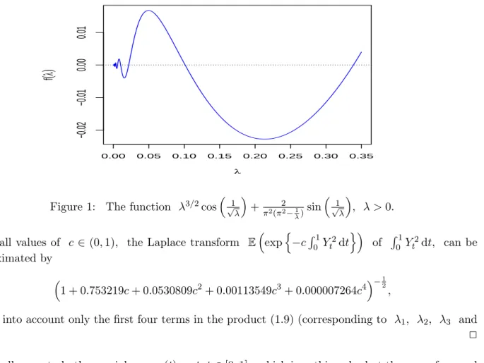
In Figure 1, we plotted the left hand side of (1.10) as a function of λ∈ (0,0.35). Hence, by (1.9),

0.00 0.05 0.10 0.15 0.20 0.25 0.30 0.35

−0.02−0.010.000.01

λ

f

(

λ

)

Figure 1: The function λ^3/2cos √1

λ

+_π2(π²₂₋1 λ)sin

√1 λ

, λ >0.

for small values of c∈ (0,1), the Laplace transform E

expn

−cR1

0 Y_t²dto

of R1

0 Y_t²dt, can be approximated by

1 + 0.753219c+ 0.0530809c²+ 0.00113549c³+ 0.000007264c⁴−¹₂

,

taking into account only the first four terms in the product (1.9) (corresponding to λ₁, λ₂, λ₃ and

λ4). 2

Finally, we study the special case g(t) :=t,t∈[0,1], which is nothing else but the case of a usual Wiener bridge over [0,1] from 0 to 0. Note that the KL expansion of a Wiener bridge has been known for a long time, see, e.g., Deheuvels [12, Remark 1.1].

1.9 Corollary. If g(t) := t, t∈ [0,1], then in the KL expansion (1.3) of the Wiener bridge Yt = Bt−tB1, t∈[0,1], the non-zero (and hence positive) eigenvalues are the solutions of the equation

sin 1

√λ

= 0, i.e., λ= 1

(kπ)², k∈N, (1.12)

and the corresponding normed eigenfunctions take the form e(t) =±√

2 sin(kπt), t∈[0,1], (1.13)

satisfying R1

0(e(t))²dt= 1.

The proof of Corollary 1.9 can be found in Section 2.

2 Proofs

Proof of Proposition 1.1. The fact that Y is a zero-mean Gauss process with continuous sample paths almost surely follows from its definition. Indeed, since for all 06t1 < t2 <· · ·< tn, n∈N,







 Yt1

... Y_tn









=















1 0 · · · 0 −g(t₁) 0 1 · · · 0 −g(t₂)

... ... . .. ... ... 0 0 · · · 1 −g(t_n)



































Bt1

Bt2

... B_tn R₁

0 g⁰(u) dBu



















 ,

to check that Y is a Gauss process it is enough to show that h

Bt1 · · · Btn

R1

0 g⁰(u) dBu

i

is normally distributed for all 06 t1 < t2 < · · ·< tn, n∈ N. This follows from the fact that B is a Gauss process and from the definition of R₁

0 g⁰(u) dBu taking into account that an L²-limit of normally distributed random variables is normally distributed (for a more detailed discussion on a similar procedure, see, e.g., the proof of Lemma 48.2 in Bauer [8]). Further, since Rt

0(g⁰(u))²du61, t∈[0,1], the process

Rt

0 g⁰(u) dBu

t∈[0,1] is a martingale, and consequently E R1

0 g⁰(u) dBu

= 0, yielding that E(Yt) = 0, t∈[0,1]. Moreover, for s, t∈[0,1],

R(s, t) = Cov

B_s−g(s) Z 1

0

g⁰(u) dB_u, B_t−g(t) Z 1

0

g⁰(u) dB_u

= Cov(B_s, B_t)−g(t) Cov Z s

0

1 dB_u, Z 1

0

g⁰(u) dB_u

−g(s) Cov Z 1

0

g⁰(u) dB_u, Z t

0

1 dB_u

+g(s)g(t) Cov Z 1

0

g⁰(u) dB_u, Z 1

0

g⁰(u) dB_u

=s∧t−g(t) Z s

0

g⁰(u) du−g(s) Z t

0

g⁰(u) du+g(s)g(t) Z 1

0

(g⁰(u))²du

=s∧t−g(t)g(s)−g(s)g(t) +g(s)g(t) =s∧t−g(s)g(t), where for the last but one equality we used g(0) = 0 and R1

0(g⁰(u))²du= 1. 2

Proof of Proposition 1.2. Let λ be a non-zero (and hence positive) eigenvalue of the integral operator AR. Then we have

(2.1)

Z 1 0

R(t, s)e(s) ds=λe(t), t∈[0,1], and hence

Z t 0

R(t, s)e(s) ds+ Z 1

t

R(t, s)e(s) ds=λe(t), t∈[0,1].

Then

λe(t) = Z t

0

(s−g(s)g(t))e(s) ds+ Z 1

t

(t−g(s)g(t))e(s) ds

= Z t

0

se(s) ds+t Z 1

t

e(s) ds−g(t) Z 1

0

g(s)e(s) ds, t∈[0,1].

(2.2)

The right-hand (and hence the left-hand) side of (2.2) is differentiable with respect to t, since e is continuous (see the Introduction), and, by differentiating with respect to t, we have

λe⁰(t) =te(t) + Z 1

t

e(s) ds−te(t)−g⁰(t) Z 1

0

g(s)e(s) ds, t∈[0,1], yielding that

λe⁰(t) =−g⁰(t) Z ₁

0

g(s)e(s) ds+ Z ₁

t

e(s) ds, t∈[0,1].

(2.3)

Differentiating (2.3) with respect to t yields (1.4) (the differentiation is allowed, since g is twice continuously differentiable). With the special choice t= 0 in (2.2), using that g(0) = 0 and λ >0, we have the boundary condition e(0) = 0, yielding the first part of (1.5). Further, by (2.3) with t= 1, we have

λe⁰(1) =−g⁰(1) Z 1

0

g(s)e(s) ds,

yielding the second part of (1.5).

Conversely, let us suppose that λ and e(t), t∈[0,1], satisfy (1.4) and (1.5). Then integration of (1.4) from t to 1 gives

λ Z ₁

t

e⁰⁰(s) ds=− Z ₁

t

e(s) ds− Z ₁

t

g⁰⁰(s) ds Z ₁

0

g(s)e(s) ds, t∈[0,1], i.e.,

λ(e⁰(1)−e⁰(t)) =− Z 1

t

e(s) ds−(g⁰(1)−g⁰(t)) Z 1

0

g(s)e(s) ds, t∈[0,1].

By (1.5), we have

−g⁰(1) Z 1

0

g(s)e(s) ds−λe⁰(t) =− Z 1

t

e(s) ds−(g⁰(1)−g⁰(t)) Z 1

0

g(s)e(s) ds, t∈[0,1], i.e.,

−λe⁰(t) =− Z 1

t

e(s) ds+g⁰(t) Z 1

0

g(s)e(s) ds, t∈[0,1], which is nothing else but (2.3). Integration of (2.3) from 0 to t gives

λ Z t

0

e⁰(s) ds=− Z t

0

g⁰(s) ds Z 1

0

g(s)e(s) ds+ Z t

0

Z 1 s

e(u) du

ds, t∈[0,1], i.e., by integration by parts,

λ(e(t)−e(0)) =−(g(t)−g(0)) Z ₁

0

g(s)e(s) ds+ Z _t

0

se(s) ds+t Z ₁

t

e(s) ds, t∈[0,1].

By (1.5) and using also g(0) = 0, we have λe(t) =−g(t)

Z 1 0

g(s)e(s) ds+ Z t

0

se(s) ds+t Z 1

t

e(s) ds

=−g(t) Z 1

0

g(s)e(s) ds+ Z 1

0

(s∧t)e(s) ds

= Z 1

0

((s∧t)−g(s)g(t))e(s) ds= Z 1

0

R(t, s)e(s) ds, t∈[0,1],

i.e., (2.1) holds, as desired. 2

Proof of Theorem 1.3. Letλ >0 and ebe solutions of (1.4) and (1.5), and introduce the notation

(2.4) K :=

Z 1 0

g(s)e(s)ds.

Then (1.4) and (1.5) take the form

λe⁰⁰(t) =−e(t)−Kg⁰⁰(t), t∈[0,1], (2.5)

e(0) = 0 and λe⁰(1) =−Kg⁰(1), (2.6)

respectively. These are, strictly speaking, not equations for the unknown functioneand scalarλ, since eis hidden also in the coefficientK. However, it will prove convenient to consider (2.5) temporarily as a second-order linear differential equation (DE) for e. The general solution of the homogeneous part of (2.5) is

e(t) =c₁cos t

√ λ

+c₂sin t

√ λ

, t∈[0,1],

where c1, c2 ∈ R. To find the solution of the inhomogeneous equation (2.5), we use the method of variation of parameters, i.e., we are looking forein the form

(2.7) e(t) =c₁(t) cos

t

√λ

+c₂(t) sin t

√λ

, t∈[0,1],

with some twice continuously differentiable functions c1, c2 : [0,1] → R. From this, we obtain the system of equations

cos t

√ λ

c⁰₁(t) + sin t

√ λ

c⁰₂(t) = 0

−sin t

√ λ

c⁰₁(t) + cos t

√ λ

c⁰₂(t) =−K

√ λg⁰⁰(t)

forc⁰₁(t) and c⁰₂(t). Solving this and substituting the solutions into (2.7), we obtain e(t) =c₁cos

t

√ λ

+c₂sin t

√ λ

+ K

√ λcos

t

√ λ

Z t 0

g⁰⁰(u) sin u

√ λ

du− K

√ λsin

t

√ λ

Z t 0

g⁰⁰(u) cos u

√ λ

du, where c1,c2 ∈R. If we take into account the initial conditione(0) = 0, we can write this in the form

e(t) =c2sin t

√ λ

+ K

√ λcos

t

√ λ

Z t 0

g⁰⁰(u) sin u

√ λ

du− K

√ λsin

t

√ λ

Z t 0

g⁰⁰(u) cos u

√ λ

du, where c2 ∈ R. Applying integration by parts twice in both integrals and taking into account the condition g(0) = 0, from this we obtain

e(t) =c2sin t

√ λ

+ K

√

λg⁰(0) sin t

√ λ

−K λg(t)

+ K

λ^3/2sin t

√ λ

Z t 0

g(u) cos u

√ λ

du− K λ^3/2 cos

t

√ λ

Z t 0

g(u) sin u

√ λ

du.

With the notation A:=c₂+^√K

λg⁰(0) the first two terms can be contracted into one:

e(t) =Asin t

√ λ

−K

λg(t) + K λ^3/2 sin

t

√ λ

Z t 0

g(u) cos u

√ λ

du

− K λ^3/2 cos

t

√ λ

Z t 0

g(u) sin u

√ λ

du.

(2.8)

Now we substitute this into the definition (2.4) ofK:

K = Z 1

0

g(t)e(t)dt=A Z 1

0

g(t) sin t

√ λ

dt−K λ

Z 1 0

g(t)²dt

+ K

λ^3/2 Z 1

0

Z t 0

g(u)g(t) cos u

√ λ

sin

t

√ λ

dudt

− K λ^3/2

Z 1 0

Z t 0

g(u)g(t) sin u

√ λ

cos

t

√ λ

dudt,

where Z 1

0

Z t 0

g(u)g(t) cos u

√ λ

sin

t

√ λ

dudt

= Z 1

0

Z 1 0

g(u)g(t) cos u

√ λ

sin

t

√ λ

dudt− Z 1

0

Z 1 t

g(u)g(t) cos u

√ λ

sin

t

√ λ

du

dt

= Z 1

0

g(u) cos u

√ λ

du

Z 1 0

g(t) sin t

√ λ

dt−

Z 1 0

Z u 0

g(u)g(t) cos u

√ λ

sin

t

√ λ

dt

du

=a_g(λ)b_g(λ)−c_g(λ).

Putting all these together, we obtain the equation

(2.9) b_g(λ)A+

−1− 1 λ

Z 1 0

g(t)²dt+a_g(λ)b_g(λ)−2c_g(λ) λ^3/2

K= 0.

Now we want to substitutee into the second equation of (2.6), therefore we calculate the derivative of (2.8):

e⁰(t) = A

√ λcos

t

√ λ

−K λg⁰(t) + K

λ² cos t

√λ Z t

0

g(u) cos u

√λ

du+ K λ^3/2sin

t

√λ

g(t) cos t

√λ

+ K λ² sin

t

√ λ

Z t 0

g(u) sin u

√ λ

du− K λ^3/2 cos

t

√ λ

g(t) sin t

√ λ

= A

√ λcos

t

√ λ

−K

λg⁰(t) + K λ²cos

t

√ λ

Z t 0

g(u) cos u

√ λ

du + K

λ² sin t

√ λ

Z t 0

g(u) sin u

√ λ

du, t∈[0,1].

Substituting this into the second equation of (2.6), we get Aλ^3/2cos

1

√ λ

+Kcos 1

√ λ

Z 1 0

g(u) cos u

√ λ

du+Ksin 1

√ λ

Z 1 0

g(u) sin u

√ λ

du= 0, or, using again the notations (1.6),

(2.10) λ^3/2cos 1

√ λ

A+

ag(λ) cos 1

√ λ

+bg(λ) sin 1

√ λ

K= 0.

This, together with (2.9), yields the following homogeneous system of linear equations for the unknowns Aand K:

bg(λ)A+

−1− 1 λ

Z 1 0

g(t)²dt+ag(λ)bg(λ)−2cg(λ) λ^3/2

K= 0, λ^3/2cos

1

√ λ

A+

a_g(λ) cos 1

√ λ

+b_g(λ) sin 1

√ λ

K= 0.

(2.11)

In what follows, we show that excluding two special cases, namely, g(t) = t, t ∈ [0,1], and g(t) =−t,t∈[0,1], the function e given in (2.8) can be identically zero if and only if A=K = 0.

To prove this, it is enough to check that the functions sin

√t λ

,t∈[0,1], and

− 1

λg(t) + 1 λ^3/2sin

t

√ λ

Z t 0

g(u) cos u

√ λ

du

− 1 λ^3/2 cos

t

√ λ

Z t 0

g(u) sin u

√ λ

du, t∈[0,1], (2.12)

are linearly independent. On the contrary, let us suppose that they are linearly dependent, i.e., there exist constants A,e Ke ∈R such that Ae²+Ke² 6= 0 and

Aesin t

√ λ

+Ke − 1

λg(t) + 1 λ^3/2 sin

t

√ λ

Z t 0

g(u) cos u

√ λ

du

− 1 λ^3/2cos

t

√ λ

Z t 0

g(u) sin u

√ λ

du

!

= 0, t∈[0,1].

(2.13)

By differentiating twice, one can check that Aesin

t

√ λ

=−Ke g⁰⁰(t)− 1

λg(t) + 1 λ^3/2sin

t

√ λ

Z t 0

g(u) cos u

√ λ

du

− 1 λ^3/2 cos

t

√ λ

Z t 0

g(u) sin u

√ λ

du

!

, t∈[0,1].

(2.14)

Comparing (2.13) and (2.14), we have Kge ⁰⁰(t) = 0, t ∈ [0,1]. If Ke = 0, then sin √t

λ

= 0, t ∈ [0,1], which is a contradiction. Thus Ke 6= 0, and we have g⁰⁰(t) = 0, t ∈ [0,1]. Using that g(0) = 0 and R1

0(g⁰(t))²dt= 1, we get g(t) =t,t∈[0,1] or g(t) =−t,t∈[0,1], which cases were excluded. This leads us to a contradiction.

Hence, excluding the two special cases g(t) =t,t∈[0,1], and g(t) =−t,t∈[0,1], we see thate is not identically zero if and only if at least one of the two coefficientsAand K is different from zero, i.e., the system (2.11) has a nontrivial solution forAand K. This is equivalent to the condition that its determinant is zero, which in turn yields equation (1.7).

If g(t) =t,t∈[0,1], or g(t) =−t,t∈[0,1], then, by integration by parts, we have

− 1

λg(t) + 1 λ^3/2 sin

t

√ λ

Z t 0

g(u) cos u

√ λ

du− 1 λ^3/2 cos

t

√ λ

Z t 0

g(u) sin u

√ λ

du

=∓ 1

λsin t

√λ Z t

0

sin u

√λ

du+1 λcos

t

√λ Z t

0

cos u

√λ

du

=∓ 1

√ λsin

t

√ λ

, t∈[0,1], yielding that the function sin

√t λ

, t ∈ [0,1], and the function in (2.12) are linearly dependent.

Further, by (2.8), using A=c2+ ^√K

λg⁰(0) =c2±^√K

λ, we have e(t) =

A∓ K

√ λ

sin

t

√ λ

=c₂sin t

√ λ

, t∈[0,1], K =

Z 1 0

g(t)e(t) dt=±c₂ Z 1

0

tsin t

√ λ

dt=±c₂√ λ

−cos 1

√ λ

+√

λsin 1

√ λ

.

By the second equation of (2.6), we have c₂√ λcos

√1 λ

=∓K (which is in fact (2.10) in the special cases g(t) =t,t∈[0,1], and g(t) =−t,t∈[0,1]). This together with the above form of K, yields sin

√1 λ

= 0, i.e., λ = _(kπ)¹ 2, k ∈ N. Next we check that the equation sin √1

λ

= 0 is nothing else but the equation (1.7) in the special cases g(t) =t,t∈[0,1], and g(t) =−t, t∈[0,1]. Using integration by parts, the constants defined in (1.6) take the forms

a_g(λ) =± Z 1

0

ucos u

√ λ

du=± √

λsin 1

√ λ

+λ

cos

1

√ λ

−1

, λ >0, bg(λ) =±

Z 1 0

usin u

√ λ

du=±

−√ λcos

1

√ λ

+λsin 1

√ λ

, λ >0, cg(λ) =

Z 1 0

Z t 0

utsin u

√ λ

cos

t

√ λ

dudt

=−√ λ

Z 1 0

t²cos² t

√ λ

dt+λ

Z 1 0

tsin t

√ λ

cos

t

√ λ

dt

=−

√ λ

6 −λ^3/2 2 cos

2

√ λ

+λ(λ−1)

4 sin

2

√ λ

, λ >0.

Hence, using R₁

0(g(t))²dt=R₁

0(±t)²dt= ¹₃, the equation (1.7) takes the form λ^3/2+

√ λ

3 + 2 −

√ λ

6 −λ^3/2 2 cos

2

√ λ

+λ(λ−1)

4 sin

2

√ λ

!!

cos 1

√ λ

+

−√ λcos

1

√ λ

+λsin 1

√ λ

2

sin 1

√ λ

= 0.

By some algebraic transformations, it is equivalent to λ²sin

√1 λ

= 0. Since λ > 0, we have sin

√1 λ

= 0, yielding λ= _(kπ)¹ 2, k∈N, as desired.

All in all, for every possible g, the equation (1.7) holds. It remains to study the form of the eigenfunctions.

If a_g(λ) cos

√1 λ

+b_g(λ) sin

√1 λ

6= 0, then from the second equation of (2.11) we have

K=−

λ^3/2cos

√1 λ

A a_g(λ) cos

√1 λ

+b_g(λ) sin

√1 λ

=−Cλe ^3/2cos 1

√ λ

,

where

Ce:= A

ag(λ) cos √1

λ

+bg(λ) sin √1

λ

.

Finally, if we substitute these expressions for K and A into (2.8), then we obtain (1.8) with some appropriately chosen C∈R.

If ag(λ) cos √1

λ

+bg(λ) sin √1

λ

= 0, then we also show that e(t) =C

"

√ λcos

1

√ λ

g(t) + cos 1

√ λ

cos

t

√ λ

Z t 0

g(u) sin u

√ λ

du

−cos 1

√ λ

sin

t

√ λ

Z t 0

g(u) cos u

√ λ

du

#

, t∈[0,1], (2.15)

is a normed eigenvector corresponding to the eigenvalue λ, where C ∈ R is chosen such that R1

0(e(t))²dt= 1. Note that (2.15) is a special case of (1.8). By Proposition 1.2, it is enough to verify that e(t), t∈[0,1], given in (2.15) satisfies (1.4) and (1.5). First, note that, by integration by parts, one can calculate

Z 1 0

g(s)e(s) ds=C √

λ Z 1

0

(g(s))²ds−ag(λ)bg(λ) + 2cg(λ)

cos 1

√ λ

.

Further,

e⁰(t) =C

"

√ λcos

1

√λ

g⁰(t)− 1

√λcos 1

√λ

sin t

√λ Z t

0

g(u) sin u

√λ

du

− 1

√ λcos

1

√ λ

cos

t

√ λ

Z t 0

g(u) cos u

√ λ

du

#

, t∈[0,1], and

e⁰⁰(t) =C

"

√ λcos

1

√ λ

g⁰⁰(t)− 1

√ λcos

1

√ λ

g(t)− 1 λcos

1

√ λ

cos

t

√ λ

Z t 0

g(u) sin u

√ λ

du

+ 1 λcos

1

√ λ

sin

t

√ λ

Z t 0

g(u) cos u

√ λ

du

#

, t∈[0,1], yielding that

λe⁰⁰(t) +e(t) =Cλ^3/2cos 1

√ λ

g⁰⁰(t), t∈[0,1].

Hence, taking into account that C6= 0, to verify (1.4) it remains to check that λ^3/2cos

1

√λ

g⁰⁰(t) =− √

λ Z 1

0

(g(s))²ds−ag(λ)bg(λ) + 2cg(λ)

cos 1

√λ

g⁰⁰(t), t∈[0,1], which is equivalent to

g⁰⁰(t)

λ^3/2+

√ λ

Z 1 0

(g(s))²ds−ag(λ)bg(λ) + 2cg(λ)

cos 1

√ λ

= 0, t∈[0,1].

(2.16)

Taking into account (1.7) and that ag(λ) cos √1

λ

+bg(λ) sin √1

λ

= 0, we have

λ^3/2+

√ λ

Z 1 0

(g(s))²ds−ag(λ)bg(λ) + 2cg(λ)

cos 1

√ λ

= 0, (2.17)

yielding (2.16). The boundary conditions (1.5) hold as well. Indeed, the boundary condition e(0) = 0 is satisfied, since g(0) = 0, and the boundary condition λe⁰(1) =−g⁰(1)R₁

0 g(s)e(s) ds is equivalent to

cos 1

√ λ

"

g⁰(1)

λ^3/2+

√ λ

Z 1 0

(g(s))²ds−a_g(λ)b_g(λ) + 2c_g(λ)

−√ λ

a_g(λ) cos 1

√ λ

+b_g(λ) sin 1

√ λ

#

= 0,

which is satisfied due to (2.17). 2

An example for the assertion in Remark 1.4. Let g : [0,1] → R, g(t) := ²

√2

π sin ^πt₂ , t ∈ [0,1]. Then g(0) = 0, g⁰(1) = 0, R1

0(g⁰(t))²dt = 1, and 0 is an eigenvalue of A_R with

−g⁰⁰(t) = ^√π

2sin ^πt₂

as an eigenfunction corresponding to 0, which is in accordance with Nazarov [21, Corollary 2]. Indeed,

Z 1 0

R(t, s)e(s) ds= Z 1

0

s∧t− 8

π²sinπs 2

sin

πt 2

π

√2sinπs 2

ds

= π

√ 2

"

Z t 0

ssin πs

2

ds+t Z 1

t

sin πs

2

ds− 8 π² sin

πt 2

Z 1 0

sin² πs

2

ds

#

= 0.

2 First proof of Corollary 1.7. We will apply Theorem 1.3 with the function g : [0,1] → R, g(t) :=

√2

π sin(πt), t∈[0,1]. First, we check that λ= _π¹2 cannot be an eigenvalue. On the contrary, let us suppose that _π¹2 is an eigenvalue. Then the constants defined in (1.6) with λ= _π¹2 take the forms

ag

1 π²

=

√ 2 π

Z 1 0

sin(πu) cos(πu) du= 0, bg

1 π²

=

√ 2 π

Z 1 0

sin²(πu) du= 1

√ 2π, cg

1 π²

= 2 π²

Z 1 0

Z t 0

sin²(πu) sin(πt) cos(πt) du

dt=− 3 8π³. Hence, using R1

0(g(t))²dt= _π²2

R1

0 sin²(πt) dt= _π¹2, (1.7) with λ= _π¹2 would imply that 1

π³ + 1 π³ − 3

4π³

(−1) + 1

2π² ·0 = 0, which leads us to a contradiction.

Using λ6= _π¹2 and the addition formulas for cosine and sine, the constants defined in (1.6) take the forms

ag(λ) =

√ 2 π

Z 1 0

sin(πu) cos u

√ λ

du= 1

√ 2π

Z 1 0

"

sin

π+ 1

√ λ

u

+ sin

π− 1

√ λ

u

# du

=

√2 π²− ¹_λ

1 + cos

1

√ λ

, λ >0, λ6= 1 π²,

bg(λ) =

√ 2 π

Z 1 0

sin(πu) sin u

√ λ

du= 1

√ 2π

Z 1 0

"

cos

π− 1

√ λ

u

−cos

π+ 1

√ λ

u

# du

=

√2 π²−¹_λ sin

1

√ λ

, λ >0, λ6= 1 π², and

cg(λ) = 2 π²

Z 1 0

Z t 0

sin(πu) sin(πt) sin u

√ λ

cos

t

√ λ

dudt

= 1 π²

Z 1 0

sin(πt) cos t

√ λ



 sin

π−^√1

λ

t π−^√1

λ

− sin

π+^√1

λ

t π+^√1

λ



dt

= 1

2π² π−^√1

λ

Z 1

0

sin

π+ 1

√ λ

t

+ sin

π− 1

√ λ

t

sin

π− 1

√ λ

t

dt

− 1

2π²

π+^√1

λ

Z 1

0

sin

π+ 1

√ λ

t

+ sin

π− 1

√ λ

t

sin

π+ 1

√ λ

t

dt

= 1 2π²

"

1 π−^√1

λ

Z ₁

0

sin²

π− 1

√ λ

t

dt− 1 π+^√1

λ

Z ₁

0

sin²

π+ 1

√ λ

t

dt

+

√2 λ

π²−_λ¹ Z 1

0

sin

π− 1

√λ

t

sin

π+ 1

√λ

t

dt

#

= 1

2π² π²−_λ¹

"

√1

λ+ π² π²−_λ¹ sin

2

√ λ

#

, λ >0, λ6= 1 π².

Hence, using R1

0(g(t))²dt= _π¹2, the equation (1.7) with λ6= _π¹₂ takes the form λ^3/2+

√λ

π² + 1

π² π²−_λ¹

√1

λ+ π² π²−_λ¹ sin

2

√ λ

!!

cos 1

√ λ

+ 2

π²−_λ¹2 sin³ 1

√ λ

= 0, λ >0, λ6= 1 π². and, by some algebraic transformations, we have

λ^3/2 π²−¹_λ cos

1

√ λ

+ 2

π² π²−¹_λ2 sin 1

√ λ

= 0, λ >0, λ6= 1 π².

By multiplying this equation with π²−_λ¹, we obtain that the equation (1.7) with λ6= _π¹2 is equivalent to (1.10).

Further, the normed eigenfunctions (1.8) with λ6= _π¹2 take the form e(t) =C

"√

2 π

√ λcos

1

√ λ

sin(πt) +

√2 π²−_λ¹

1 + cos

1

√ λ

cos

1

√ λ

+ sin²

1

√ λ

sin

t

√ λ

+

√2 π cos

1

√ λ

cos

t

√ λ

Z t 0

sin(πu) sin u

√ λ

du

−

√ 2 π cos

1

√ λ

sin

t

√ λ

Z t 0

sin(πu) cos u

√ λ

du

#

=C

"√

2 π

√ λcos

1

√ λ

sin(πt) +

√2 π²−_λ¹

1 + cos

1

√ λ

sin

t

√ λ

+ 1

√ 2π cos

1

√ λ

cos

t

√ λ



 sin

π−^√1

λ

t

π−^√1

λ

− sin

π+^√1

λ

t

π+^√1

λ





− 1

√2π cos 1

√ λ

sin

t

√ λ



−

cos π+^√1

λ

t π+^√1

λ

− cos

π− ^√1

λ

t π− ^√1

λ

+ 1

π+^√1

λ

+ 1

π−^√1

λ





#

=C

"√

2 π

√ λcos

1

√ λ

sin(πt) +

√2 π²−_λ¹ sin

t

√ λ

+ 1

√ 2π

π−^√1

λ

cos 1

√

λ sin

π− 1

√ λ

t

cos

t

√ λ

+ cos

π− 1

√ λ

t

sin

t

√ λ

+ 1

√2π π+^√1

λ

cos 1

√

λ sin t

√ λ

cos

π+ 1

√ λ

t

−cos t

√ λ

sin

π+ 1

√ λ

t

#

=C

"√

2 π

√ λcos

1

√λ

sin(πt) +

√ 2 π²−_λ¹ sin

t

√λ

+ 1

√2π π−^√1

λ

cos 1

√ λ

sin(πt) + 1

√2π π+^√1

λ

cos 1

√ λ

sin(−πt)

#

= C√ 2 π²−_λ¹

sin

t

√ λ

+

√ λπcos

1

√ λ

sin(πt)

,

where C∈R is such that R1

0(e(t))²dt= 1. Hence 1

C² = 2 π²−_λ¹2

Z 1 0

sin²

t

√ λ

+λπ²cos² 1

√ λ

sin²(πt) + 2

√ λπcos

1

√ λ

sin

t

√ λ

sin(πt)

dt

= 2

π²−_λ¹2

λπ² 2 cos²

1

√λ

+

√

λ π² π²−_λ¹ −1

4

! sin

2

√λ

+1 2

! .