Perturbed Li–Yorke homoclinic chaos

Perturbed Li–Yorke homoclinic chaos

Marat Akhmet

, Michal Feˇckan

, Mehmet Onur Fen

and Ardak Kashkynbayev

1Department of Mathematics, Middle East Technical University, 06800 Ankara, Turkey

2Department of Mathematical Analysis and Numerical Mathematics, Comenius University in Bratislava, Mlynská dolina, 842 48 Bratislava, Slovakia

3Mathematical Institute of Slovak Academy of Sciences, Štefánikova 49, 814 73 Bratislava, Slovakia

4Department of Mathematics, TED University, 06420 Ankara, Turkey

5Department of Mathematics, School of Science and Technology, Nazarbayev University, 010000 Astana, Kazakhstan

Received 3 May 2018, appeared 4 September 2018 Communicated by Eduardo Liz

Abstract. It is rigorously proved that a Li–Yorke chaotic perturbation of a system with a homoclinic orbit creates chaos along each periodic trajectory. The structure of the chaos is investigated, and the existence of infinitely many almost periodic orbits out of the scrambled sets is revealed. Ott–Grebogi–Yorke and Pyragas control methods are utilized to stabilize almost periodic motions. A Duffing oscillator is considered to show the effectiveness of our technique, and simulations that support the theoretical results are depicted.

Keywords: homoclinic orbit, Li–Yorke chaos, almost periodic orbits, Duffing oscillator.

2010 Mathematics Subject Classification: 34C28, 34C37, 34H10.

1 Introduction

Traditionally, analysis of nonlinear dynamical systems has been restricted to smooth problems, that is, to smooth differential equations. Besides stability analysis of fixed points and periodic orbits, another fascinating phenomenon is the existence of chaotic orbits. The presence of such orbits has the consequence that the motions of the system depend sensitively on initial conditions, and the behavior of orbits in the future is unpredictable. Such a chaotic behavior of solutions can be explained mathematically by showing the existence of a transverse homoclinic point of the time map with the corresponding invariant Smale horseshoe [21,33,34]. In general, however, it is not easy to demonstrate the existence of a transverse homoclinic point. The perturbation approach, which is now known as the Melnikov method, is a powerful tool for that purpose [17–19]. The starting point is a nonautonomous system, the unperturbed system/equation, with a (necessarily) nontransverse homoclinic orbit. It is known that if we set up a perturbed system by adding a periodic (or almost periodic) perturbation of a

BCorresponding author. Email: marat@metu.edu.tr

sufficiently small amplitude to the unperturbed system and a certain Melnikov function has a simple zero at some point, then the perturbed system has a transverse homoclinic point with the corresponding Smale horseshoe [11].

Endogenously generated chaotic behavior of systems are well investigated in the litera- ture. The systems of Lorenz [28], Rössler [36] and Chua [13–15] as well as the Van der Pol [12,24,25] and Duffing [29,31,41,42] oscillators can be considered as systems which are ca- pable of generating chaos endogenously. Chaotification of systems with asymptotically stable equilibria through different types of perturbations can be found in the papers [1–3] and the book [5]. Moreover, the study [4] is concerned with the existence of homoclinic and hetero- clinic motions in economic models perturbed with exogenous shocks. In the present study, we consider a system with a homoclinic solution under the influence of a chaotic forcing term.

The formation of exogenous chaos is theoretically investigated. Our results are based on the Li–Yorke definition of chaos [27] in a modified sense that was introduced in the papers [6,8].

To emphasize the role of the homoclinic solution in the paper, we call the dynamics Li-*Yorke homoclinic chaos. An example based on Duffing oscillator is presented to show the effective- ness of our results. Moreover, the controllability of the obtained chaos is shown by means of the Ott–Grebogi–Yorke (OGY) [32] and Pyragas [35] control methods.

Our suggested results are of a significant interest due to the theoretical importance and perspectives for applications. This is the first time in the literature that chaos is obtained as a union of infinitely many sets of chaotic motions for a single equation by means of a perturbation. It was observed from experimental data that chaos is a positive factor for brain activities [39] as well as for robotic dynamics [30,40]. This is the reason why the presence of infinitely many sets of chaotic motions in the dynamics of a single equation may shed light on the capacity of the brain and provide an opportunity for new designs in robotics.

In the next section, we will introduce the systems which are the main objects of our inves- tigation and will give information concerning their properties under some conditions.

2 The model

Let A be an equicontinuous family of functions defined on R with range Λ, where Λ is a compact subset ofR^m. In order to generate chaos, we perturb the system

z⁰ = f(z,t) (2.1)

with the elements of the familyA and set up the system

u⁰ = f(u,t) +h(x(t))_{, (2.2)} where x(t) ∈_A, the function f : Rⁿ×_R → _Rⁿ is twice continuously differentiable in uand continuous int, and the function h:Λ→_Rⁿis continuous.

In the remaining parts of the paper, we will make use of the usual Euclidean norm for vectors and the norm induced by the Euclidean norm for matrices.

The following conditions are required.

(C1) f(u,t+1) = f(u,t)for all u∈_Rⁿandt ∈_R;

(C2) There exist positive numbersL₁andL2such that

L₁kx₁−x₂k ≤ kh(x₁)−h(x₂)k ≤L₂kx₁−x₂k for allx₁, x₂∈ _Λ.

We suppose that system (2.1) has a hyperbolic periodic solution p(t) with a homoclinic solution q(t)such that the variational equation w⁰ = Duf(q(t),t)whas only the zero solution bounded on the real axis. Under this assumption, it is known thatq(t)is a transversal homo- clinic orbit, i.e., the 1-time map G:Rⁿ→_Rⁿof system (2.1) has a hyperbolic fixed pointp(0) with a transversal homoclinic orbit {q(j)}_j∈Z. Following Sections 3 and 4 of [33], especially Theorem 4.8 of [33], we get a collection of uniformly bounded solutions

ν_β(t)

β∈Sσ of system (2.1) orbitally near q(t), where the index set Sσ,σ ≥ 2, is the set of doubly infinite sequences d = . . . ,d−1,d₀,d₁, . . .

with d_i ∈ {1, . . . ,σ} for alli ∈ _{Z, i.e.,} S_σ = {1, 2, . . . ,σ}^Z such that each linear system

w⁰ =Duf(ν_β(t),t)w (2.3) has an exponential dichotomy onRwith uniform positive constantsK andα, and projections Q_β:

W_β(t)Q_βW_β⁻¹(s)≤ Ke^−α(t−s) for all t,s, t≥s,

W_β(t)(I−Q_β)W_β⁻¹(s)≤ Ke^α(t−s) for all t,s, t≤s, (2.4) whereIis then×nidentity matrix andW_βis the fundamental matrix of system (2.3) satisfying W_β(0) = I. It is worth noting that system (2.2) may not possess a homoclinic solution.

By Theorem 4.8 of [33], an iterativeG^k0, for some fixedk0∈N, is conjugate to the Bernoulli shift on an invariant compact subset H ⊂ _Rⁿ, G^k0 : H → _H. So G^k0 hasi-periodic orbits in H for any natural number i. This gives that the map G has periodic orbits with periods ik₀ starting in H. Since by definition ν_β(0) = ς_β for some ς_β ∈ _H and then G^j(ς_β) = ν_β(j) for any j∈ Z, we see that among these ν_β(t) there areik₀-periodic solutions of (2.1) for any i∈_N. In what follows we will denote byP_σ⊂ S_σ,σ≥2, the index set for which the bounded solutions

ν_β(t)

β∈P_σ of system (2.1) are periodic.

3 Bounded solutions

Introducing the new variable y throughy = u−ν_β(t), β ∈ S_σ, system (2.2) can be written in the form

y⁰ = D_uf(ν_β(t),t)y+F_β(y,t) +h(x(t)), (3.1) where the function F_β :Rⁿ×_R→_Rⁿis defined as

Fβ(y,t) = f(y+ν_β(t),t)− f(ν_β(t),t)−Duf(ν_β(t),t)y. (3.2) Using the dichotomy theory [16], one can verify that for a fixed x(t) ∈ _A, a function y(t)which is bounded on the real axis is a solution of system (3.1) if and only if the integral equation

y(t) =

Z _∞

−_∞G_β(t,s)[F_β(y(s),s) +h(x(s))]ds (3.3) is satisfied, where

G_β(t,s) =

(W_β(t)Q_βW_β⁻¹(s)_, t >s,

−W_β(t)(I−Q_β)W_β⁻¹(s), t <s. (3.4) Since f is twice continuously differentiable in u, under the condition (C1), there exist positive numbers N₁and N2such that

sup

t∈_R, β∈Sσ

D_uf(ν_β(t),t) ≤N₁

and

sup

t∈_R,β∈Sσ

Duuf(ν_β(t),t)≤ N2

for each bounded solutionν_β(t), β∈ S_σ, of (2.1).

The following condition is also required.

(C3) M_h < ^α

2

16K²N₂, whereM_h =sup

x∈_Λ

kh(x)k. Under the condition(C3), let us denote

R₀ = ^α−^pα²−16K²N₂M_h

4KN₂ .

The following lemma is concerned with the existence and uniqueness of bounded solutions of system (3.1).

Lemma 3.1. Suppose that the conditions(C1)–(C3)hold. For each x(t)∈_A system(3.1)possesses a unique solutionφ^β_x(t)(t),β∈Sσ,which is bounded on the real axis such thatsup_t∈R

φ^β_x(t)(t)≤ R₀. Proof. LetC₀ be the set of uniformly bounded, continuous functionsw(t):R→_Rⁿsatisfying kwk_∞ ≤R0, where the normk·k_∞ is defined by

kwk_∞ =_sup

t∈Rkw(t)k. (3.5)

One can confirm thatC₀ is complete with the metric induced by the normk·k_∞.

Fix an arbitrary functionx(t)∈_A and define an operatorΠonC₀ through the equation Πw(t) =

Z _∞

−_∞G_β(t,s)[F_β(w(s),s) +h(x(s))]ds, (3.6) where F_β and G_β are defined by (3.2) and (3.4), respectively. Let w(t)belong to C₀. One can obtain for eacht∈_Rthat

kF_β(w(t),t)k ≤ kw(t)k

Z ₁

0

D_uf(θw(t) +ν_β(t),t)−D_uf(ν_β(t),t)dθ

≤ kw(t)k²

Z ₁

0

Z ₁

0

D_uuf(τθw(t) +ν_β(t),t)dτdθ

≤ N₂kw(t)k².

(3.7)

The inequality (3.7) yields

k_Πwk_∞ ≤ ^2K(N₂kwk²_∞+M_h) α ≤R₀, and therefore,Π(C₀)⊆ C₀.

Now, suppose thatw₁(t)_andw₂(t)belong to the setC₀. It can be verified that Πw1(t)−_Πw2(t) =

Z _∞

−_∞Gβ(t,s)Feβ(w₁(s),w2(s),s)ds, where the functionFe_β :Rⁿ×_Rⁿ×_R→_Rⁿ is defined through the equation

Fe_β(z₁,z₂,t) = f(z₁+ν_β(t)_,t)− f(z₂+ν_β(t)_,t)−D_uf(ν_β(t)_,t)(z₁−z₂)_{. (3.8)}

For eacht∈R, we have that kFe_β(w₁(t),w2(t),t)k

≤ kw₁(t)−w₂(t)k

Z ₁

0

D_uf(θw₁(t) + (1−θ)w₂(t) +ν_β(t),t)−D_uf(ν_β(t),t)dθ

≤ kw₁(t)−w₂(t)k

Z ₁

0

Z ₁

0

D_uuf(τ(θw₁(t) + (₁−θ)w₂(t)) +ν_β(t)_,t)

×(θkw₁(t)k+ (1−θ)kw2(t)k)dτdθ

≤ kw₁(t)−w2(t)kmax{kw₁(t)k,kw2(t)k}

×

Z ₁

0

Z ₁

0

D_uuf(τ(θw₁(t) + (1−θ)w₂(t)) +ν_β(t),t)dτdθ

≤N₂kw₁(t)−w₂(t)kmax{kw₁(t)k,kw₂(t)k}.

(3.9)

One can confirm using the last inequality that k_Πw1−_Πw2k_∞ ≤ ^2KN2R0

α kw₁−w₂k_∞ < ¹

2kw₁−w₂k_∞.

Hence, the operatorΠis a contraction. Consequently, for eachx(t)∈_A, there exists a unique solutionφ_x^β_(t)(t)of system (3.1) which is bounded on the real axis such that sup_t∈R

φ_x^β_(t)(t)≤ R₀.

4 Li–Yorke chaos

In the pioneer paper [27], chaos is considered with infinitely many periodic solutions sep- arated from the elements of a scrambled set. In the present study, we will make use of a modified version of Li–Yorke chaos such that infinitely many almost periodic motions take place in the dynamics instead of periodic ones. Such a modification was first considered in the paper [8]. Since the concept of chaotic set of functions will be used in the theoretical dis- cussions, let us explain the ingredients of Li–Yorke chaos with infinitely many almost periodic motions [6–8].

Let Γ be a set of uniformly bounded functions ψ : R → _R^r. A couple of functions ψ(t),ψ(t) ∈ _Γ×_Γ is called proximal if for an arbitrary small number e > 0 and an ar- bitrary large number E > 0 there exists an interval J ⊂ _R with a length no less than E such that

ψ(t)−ψ(t) < e for all t ∈ J. Besides, a couple of functions ψ(t),ψ(t) ∈ _Γ×_Γ is frequently (e₀,∆)-separated if there exist numberse₀ >0, ∆> 0 and infinitely many disjoint intervals each with a length no less than∆such that

ψ(t)−ψ(t)>e₀ for eachtfrom these intervals. It is worth noting that the numberse0and∆may depend on the functionsψ(t)and ψ(t).

We say that a couple of functions ψ(t),ψ(t)∈_Γ×_Γis a Li–Yorke pair if they are proximal and frequently(e0,∆)-separated for some positive numberse0and∆.

The description of a Li–Yorke chaotic set with infinitely many almost periodic motions is given in the next definition [6–8].

Definition 4.1. Γis called a Li–Yorke chaotic set with infinitely many almost periodic motions if:

(i) there exists a countably infinite setC ⊂ _Γof almost periodic functions;

(ii) there exists an uncountable set U ⊂ Γ, the scrambled set, such that the intersection of U andC is empty and each couple of different functions inside U ×_U is a Li–Yorke pair;

(iii) for any function ψ(t) ∈ _U and any almost periodic function ψ(t) ∈ _C, the couple ψ(t),ψ(t) is frequently(e₀,∆)−separated for some positive numberse₀ and∆.

In order to study the existence of chaos theoretically in the dynamics of system (2.2), let us introduce the sets of functions

Bβ =ⁿφ_x^β_(t)(t): x(t)∈_A^o, β∈Sσ. (4.1) Lemma 4.2. Under the conditions (C1)–(C3), if a couple (x(t)_,x(t)) ∈ _A ×_A is proximal, then the same is true for the couple φ^β_x(t)(t),φ^β_x(t)(t) ∈_Bβ×_Bβ, β∈ Sσ.

Proof. Fix an arbitrary small positive numbere, and letµbe a number such that µ≥1+ ^2KL2

α−2KN₂R₀.

Suppose thatEis an arbitrary large positive number satisfyingE> ¹

δln ^2H_e^0µ

, where δ= ^pα²−2KN₂R₀α

and

H0= 2

α−^pα²−2KN2R0α

M_h+N2R²₀

αN₂R₀ .

Because the couple (x(t),x(t)) ∈ _A ×_A is proximal, there exist a real number a₀ and a numberE0≥ Esuch that the inequalitykx(t)−x(t)k< _µ^e holds for allt∈ [a0,a0+3E0].

The bounded solutionsφ^β_x(t)(t)andφ^β_x(t)(t)of system (3.1) satisfy the relation φ^β_x(t)(t)−φ_x^β_(t)(t) =

Z _∞

−_∞G_β(t,s)Fe_β

φ_x^β_(t)(s),φ_x^β_(t)(s),s

+h(x(s))−h(x(s))ds,

where the functionsG_β and Fe_β are defined by (3.4) and (3.8), respectively. According to (3.9) we have fort ∈_Rthat

Fe_β

φ^β_x(t)(t),φ_x^β_(t)(t),t

≤N₂R₀

φ^β_x(t)(t)−φ_x^β_(t)(t)

≤2N₂R²₀. (4.2) Making use of the inequality (4.2) it can be verified for t∈ [a₀,a₀+3E₀]that

φ^β_x(t)(t)−φ_x^β_(t)(t)

≤ ^2KL2e

µα +^2K(M_h+N₂R²₀) α

e^{−α(t−a0)}+e^{−α(a0+3E0−t)} +KN2R0

Z _a0+3E0

a0

e^−α|t−s|

φ^β_x(t)(s)−φ_x^β_(t)(s) ds.

Now, we obtain by applying TheoremA.1given in the Appendix that

φ^β_x(t)(t)−φ_x^β_(t)(t)

≤ ^2KL2e

µ(α−2KN₂R₀)+H₀

e^{−δ(t−a0)}+e^{−δ(a0+3E0−t)} .

SinceE> ¹

δln ^2H_e^0µ

, the inequality H₀

e^{−δ(t−a0)}+e^{−δ(a0+3E0−t)}

< ^e µ

is valid for t ∈ J, where J = [a0+E0,a0+2E0]. Thus, if t belongs to the interval J, then we have that

φ_x^β_(t)(t)−φ^β_x(t)(t)<

1+ ^2KL2 α−2KN2R0

e

µ

≤e.

Consequently, the couple φ_x^β_(t)(t),φ^β_x(t)(t) ∈_Bβ×_Bβ is proximal.

Remark 4.3. The interval J mentioned in the proof of Lemma4.2is uniform for each β∈ Sσ. The next assertion is concerned with the second ingredient, the frequent separation feature, of Li–Yorke chaos.

Lemma 4.4. Assume that the conditions (_C1)_–(_C3) hold. If a couple (x(_t)_,x(_t)) ∈ _A ×_A is frequently(e₀,∆)-separated for some positive numberse₀and∆, then the couple φ^β_x(t)(t),φ^β_x(t)(t)∈ Bβ×_Bβ is frequently(e₁,∆)-separated for some positive numberse₁and∆uniform for eachβ∈ Sσ. Proof. Because the couple (x(t),x(t)) ∈ _A ×_A is frequently (e₀,∆)-separated, there exist infinitely many disjoint intervals J_k, k ∈ _N, each with a length no less than ∆ such that kx(t)−x(t)k>e0for each tfrom these intervals.

Suppose thath(x) = (h₁(x),h₂(x), . . . ,h_n(x)), where eachh_j,j=1, 2, . . . ,n, is a real valued function. The function eh : Λ×_Λ → _Rⁿ defined by eh(z₁,z₂) = h(z₁)−h(z₂) is uniformly continuous onΛ×_{Λ. SinceA} is an equicontinuous family onR, the set of functions whose elements are of the form h_j(x(t))−h_j(x(t)), j = 1, 2, . . . ,n, where x(t),x(t) ∈ _A, is also an equicontinuous family onR. Therefore, there exists a positive numberτ<∆, which does not depend on the functions x(t) and x(t), such that for every t₁,t₂ ∈ _R with |t₁−t₂| < τ, the inequality

h_j(x(t₁))−h_j(x(t₁))− h_j(x(t₂))−h_j(x(t₂))< ^L1e0 2√

n (4.3)

holds for all j=1, 2, . . . ,n.

Fix a natural number k. Let us denote ξ_k = η_k−_{τ/2, where} η_k is the midpoint of the interval J_k. There exists an integerj_k, 1≤j_k ≤n, such that

h_jk(x(η_k))−h_jk(x(η_k)) ≥ √^L1

n kx(η_k)−x(η_k)k> ^L√^1e0

n. (4.4)

For t∈[ξ_k,ξ_k+τ], one can confirm by means of (4.3) that

h_jk(x(η_k))−h_jk(x(η_k))−h_jk(x(t))−h_jk(x(t)) < ^L1e0 2√

n. Accordingly, the inequality (4.4) yields

h_jk(x(t))−h_jk(x(t))> ^L1e0 2√

n, t∈ [ξ_k,ξ_k+τ].

Since there exist numbersc₁,c₂, . . . ,c_n∈ [ξ_k,ξ_k+τ]such that the equation

Z _ξk+τ ξ_k

(h(x(s))−h(x(s)))ds

=τ

∑

h_j(x(c_j))−h_j(x(c_j))²

!1/2

, is valid, we have

Z _ξk+τ

ξ_k

(h(x(s))−h(x(s)))ds

≥τ

h_jk(x(c_jk))−h_jk(x(c_jk)) > ^τL1e0 2√

n . (4.5)

The bounded solutionsφ^β_x(t)(t)andφ^β_x(t)(t)satisfy the equation φ_x^β_(t)(t)−φ_x^β_(t)(t) =φ^β_x(t)(ξ_k)−φ^β_x(t)(ξ_k)

+

Z _t

ξ_k

h Fe_β

φ^β_x(t)(s),φ_x^β_(t)(s),s

+D_uf(ν_β(s),s)φ_x^β_(t)(s)−φ^β_x(t)(s)ⁱds +

Z _t

ξ_k

(h(x(s))−h(x(s)))ds,

where the function Fe_β is defined by (3.8). Therefore, making use of the inequalities (4.2) and (4.5) we obtain that

φ^β_x(t)(ξ_k+τ)−φ_x^β_(t)(ξ_k+τ)

> ^τL1e0 2√

n −[1+ (N₁+N2R0)τ] max

t∈[ξ_k,ξ_k+τ]

φ_x^β_(t)(t)−φ^β_x(t)(t) . Hence, the inequality

t∈[maxξk,ξk+τ]

φ^β_x(t)(t)−φ_x^β_(t)(t)> ^τL1e0

2[2+ (N₁+N₂R₀)τ]√ n holds.

Now, suppose that

t∈[maxξ_k,ξ_k+τ]

φ_x^β_(t)(t)−φ^β_x(t)(t) =

φ^β_x(t)(ρ_k)−φ^β_x(t)(ρ_k)

for someρ_k ∈[ξ_k,ξ_k+τ]. Let us define the numbers

e₁= ^τL1e0

4[2+ (N₁+N₂R₀)τ]√ n and

∆=min τ

2, τL₁e0

8[2+ (N₁+N2R0)τ] [M_h+ (N₁+N2R0)R0]√ n

.

It is worth noting that e₁ and ∆ do not depend on β ∈ Sσ. Moreover, we denoteθ_k = ρ_k if ξ_k ≤ρ_k ≤ξ_k+τ/2 andθ_k = ρ_k−_∆ifξ_k+τ/2<ρ_k ≤ξ_k+τ.

Using the inequality

φ_x^β_(t)(t)−φ^β_x(t)(t)≥ φ^β_x(t)(ρ_k)−φ_x^β_(t)(ρ_k)

−

Z _t

ρk

Fe_β

φ^β_x(t)(s),φ_x^β_(t)(s),s

+Duf(ν_β(s),s)φ_x^β_(t)(s)−φ^β_x(t)(s)ds

−

Z _t

ρ_k

kh(x(s))−h(x(s))kds

together with (4.2), it can be verified fort∈ θ_k,θ_k+_∆that

φ^β_x(t)(t)−φ_x^β_(t)(t)> ^τL1e0

2[2+ (N₁+N₂R₀)τ]√

n−2[M_h+ (N₁+N₂R₀)R₀]_∆≥e₁. One can confirm that the intervals[θ_k,θ_k+_∆]_,k∈N, are disjoint. Consequently, the couple φ_x^β_(t)(t),φ_x^β_(t)(t) ∈_Bβ×_Bβ is frequently(e₁,∆)-separated uniform for eachβ∈S_σ.

Next, we deal with the almost periodic solutions of system (3.1). A continuous function ϑ: R→ _R^r is said to be almost periodic, if for anye> 0 there existsl> 0 such that for any interval with lengthlthere exists a numberT in this interval satisfyingkϑ(t+T)−ϑ(t)k<e for all t∈_R[22,26,37].

In the proof of the following assertion, we will make use of the operatorΠdefined by (3.6).

Lemma 4.5. Suppose that the conditions (C1)–(C3)are satisfied. If x(t)∈ _A is an almost periodic function, then the bounded solutionφ_x^β_(t)(t),β∈ P_σ, of system(3.1)is also almost periodic.

Proof. Let us denote by C₁ the set of continuous almost periodic functions w(t) : R → _Rⁿ satisfying kwk_∞ ≤ R0, where the norm k·k_∞ is defined by (3.5). If w(t) ∈ C₁, then one can confirm using the results of [22] that the functions A_β(t) = D_uf(ν_β(t),t) and f_β(t) = F_β(w(t),t) +h(x(t))are almost periodic forβ∈ P_σ. On the other hand, according to [16, p. 72], Πw(t)is also almost periodic, whereΠis the operator defined by (3.6). Therefore,Π(C₁)⊆ C₁. Since the operatorΠis contractive as shown in the proof of Lemma3.1, its fixed pointφ_x^β_(t)(t) is almost periodic for each β∈ P_σ.

Now, we state and prove our main theorem.

Theorem 4.6. Suppose that the conditions (C1)–(C3) are valid. If the collection A is Li–Yorke chaotic with infinitely many almost periodic motions, then the same is true for each of the collections Bβ,β∈ P_σ.

Proof. LetC ⊂_A be a countably infinite set of almost periodic functions, and for eachβ∈ P_σ define the set

Cβ =ⁿφ_x^β_(t)(t): x(t)∈_C^o.

Condition (C2) implies that there is a one-to-one correspondence between the sets C and Cβ, β ∈ P_σ. Therefore, Cβ ⊂ _Bβ is also countably infinite for each β ∈ P_σ. Furthermore, Lemma4.5implies thatCβ, β∈ P_σ, consists of almost periodic functions.

Next, we denote byU ⊂_A an uncountable scrambled set. Let us introduce the sets Uβ =ⁿφ_x^β_(t)(t): x(t)∈_U^o,

where β ∈ P_σ. It can be verified using condition (C2) one more time that the sets Uβ, β∈ P_σ, are all uncountable, and no almost periodic functions take place in these sets, i.e., the intersection ofUβ andCβ is empty.

Because each couple of functions inside U ×_U is proximal, Lemma 4.2 implies that the same is true for each couple inside Uβ×_Uβ, β ∈ P_σ. On the other hand, according to Lemma 4.4, there exist positive numbers e₁ and ∆ such that each couple of functions inside Uβ×_Uβ is frequently e₁,∆

-separated. Lemma4.4also implies the presence of the frequent separation feature for each couple inside Uβ×_Cβ, β ∈ P_σ. Consequently, each of the collectionsBβ, β∈ P_σ, is Li–Yorke chaotic.

Remark 4.7. System (2.1) may possess bounded solutions other than ν_β(t)

β∈Sσ. Therefore, there may exist a chaotic set corresponding to each of such solutions, but its verification is a difficult task in general, which would require additional assumptions on the system.

It is worth noting that the criterion in Definition4.1for the existence of a countably infinite subset of almost periodic functions in a Li–Yorke chaotic can be replaced with the existence of a countably infinite subset of quasi-periodic functions [7]. In the following section, we will exemplify Li–Yorke homoclinic chaos with infinitely many quasi-periodic motions.

5 An example

This part of the paper is devoted to an illustrative example. First of all, we will take into account a forced Duffing equation, which is Li–Yorke chaotic with infinitely many quasi- periodic motions, as the source of chaotic perturbations. A relay function will be used in this equation as the forcing term to ensure the presence of chaos. Detailed theoretical as well as numerical results concerning relay systems can be found in the studies [1,2,5]. Next, to provide the Li–Yorke homoclinic chaos, we will perturb another Duffing equation, which admits a homoclinic orbit, by the solutions of the former one.

Another issue that we will focus on is the stabilization of unstable quasi-periodic motions.

In the literature, control of chaos is understood as the stabilization of unstable periodic orbits embedded in a chaotic attractor [20,38]. However, we will demonstrate the stabilization of quasi-periodic motions instead of periodic ones. The presence of chaos with infinitely many unstable quasi-periodic motions will be revealed by means of an appropriate chaos control technique based on the Ott–Grebogi–Yorke (OGY) [32] and Pyragas [35] control methods.

Let us consider the following forced Duffing equation,

x⁰⁰+0.82x⁰+1.4x+0.01x³ =0.25 sin(3t) +v(t,ζ,λ), (5.1) where the relay functionv(t,ζ,λ)is defined as

v(t,ζ,λ) =

(0.3, ifζ_2j <t≤ ζ_2j+1, j∈_Z,

1.9, ifζ_2j−1 <t≤ ζ_2j, j∈_Z. ^(5.2) In (5.2), the sequence ζ = ζ_{j j∈Z}, ζ₀ ∈ [0, 1], of switching moments is defined through the equationζ_j = j+κ_j, j∈ Z, and the sequence

κ_{j j∈Z} is a solution of the logistic map

κ_j+1=λκ_j(1−κ_j), (5.3)

whereλis a real parameter. The interval[0, 1]is invariant under the iterations of (5.3) for the values ofλbetween 1 and 4 [23], and the map possesses Li-Yorke chaos forλ=3.9 [27].

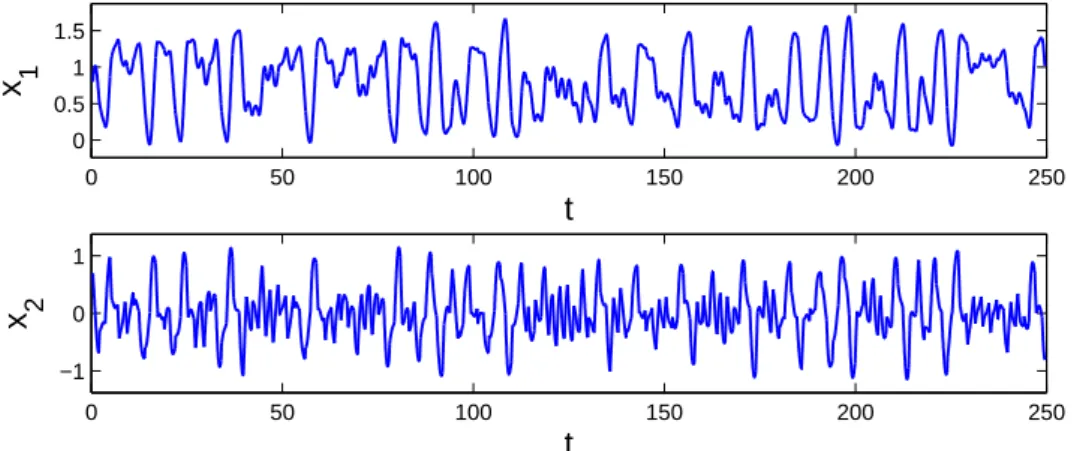
Making use of the new variables x₁ =xandx₂= x⁰, one can reduce (5.1) to the system x₁⁰ =x2

x₂⁰ =−1.4x₁−0.82x₂−0.01x₁³+0.25 sin(3t) +v(t,ζ,λ). (5.4) For each ζ₀ ∈ [_{0, 1}], system (5.4) with λ = 3.9 possesses a solution which is bounded on the whole real axis, and the collection A consisting of all such bounded solutions is Li–

Yorke chaotic with infinitely many quasi-periodic motions [2,6,7]. Moreover, for each natural numberρ, system (5.4) admits unstable periodic solutions with periods 2ρ.

Figure5.1shows the solution of system (5.4) withλ=3.9 andζ₀= 0.41 corresponding to the initial datax₁(0.41) =0.8,x2(0.41) =0.7. The simulation results seen in Figure5.1confirm the presence of chaos in (5.4).

0 50 100 150 200 250

0 0.5 1 1.5

t

x 1

0 50 100 150 200 250

−1 0 1

t

x 2

Figure 5.1: The chaotic behavior of system (5.4).

Next, let us consider the following Duffing equation [9],

z⁰⁰+0.15z⁰−0.5z(1−z²) =0.2 sin(0.9t). (5.5) It was mentioned in paper [9] that the equation (5.5) is chaotic, and it admits a homoclinic orbit.

By means of the variablesz₁ =z andz₂ = z⁰, equation (5.5) can be written as a system in the form,

z⁰₁= z₂

z⁰₂= −0.15z₂+0.5z₁(1−z²₁) +0.2 sin(0.9t). (5.6) We perturb system (5.6) with the solutions of (5.4) and set up the system

u⁰₁ =u₂+1.9(x₁(t) +0.4 sin(x₁(t)))

u⁰₂ =−0.15u₂+0.5u₁(1−u²₁) +1.3x₂(t) +0.2 sin(0.9t). (5.7) System (5.7) is in the form of (2.2) with

f(u₁,u₂,t) = ^u2

−0.15u₂+0.5u₁(1−u²₁) +0.2 sin(0.9t)

!

and

h(x₁,x2) = ^1.9(x₁+0.4 sin(x₁)) 1.3x₂

! .

According to Theorem4.6, system (5.7) possesses Li–Yorke chaos with infinitely many quasi- periodic motions.

In order to simulate the chaotic behavior, we use the solution (x₁(t)_,x₂(t)) of (5.4) which is represented in Figure5.1 as the perturbation in (5.7), and depict in Figure 5.2 the solution of (5.7) with the initial datau₁(0.41) =0.12,u₂(0.41) =0.013. Figure5.2supports the result of Theorem4.6such that the perturbed system (5.7) exhibits chaos.

0 50 100 150 200 250

−4

−2 0 2 4

t

u 1

0 50 100 150 200 250

−10

−5 0 5

t

u 2

Figure 5.2: The chaotic solution of system (5.7) with u₁(0.41) = 0.12 and u₂(0.41) = 0.013. The solution (x₁(t),x₂(t)) of (5.4), which is represented in Figure5.1, is used as the perturbation in (5.7).

Next, we depict in Figure5.3 the trajectories of (5.6) and (5.7) corresponding to the initial data z₁(0.41) = 0.12, z₂(0.41) = 0.013 and u₁(0.41) = 0.12, u₂(0.41) = 0.013, respectively.

Here, the trajectory of (5.6) is depicted in blue and the trajectory of (5.7) is shown in red. It is seen in Figure5.3 that even if the same initial data is used, systems (5.6) and (5.7) generate completely different chaotic trajectories.

−4 −3 −2 −1 0 1 2 3 4

−10

−8

−6

−4

−2 0 2 4 6

u1, z

1

u 2, z 2

Figure 5.3: Chaotic trajectories of systems (5.6) and (5.7). The trajectory of (5.6) with z₁(0.41) = 0.12, z₂(0.41) = 0.013 is represented in blue color, while the trajectory of (5.7) corresponding tou₁(0.41) =0.12,u₂(0.41) =0.013 is shown in red color. One can observe that the unperturbed system (5.6) and the perturbed system (5.7) possess different chaotic motions.

Now, we will confirm the presence of chaos with infinitely many quasi-periodic motions in the dynamics of (5.7) by stabilizing one of them through a control technique based on the OGY [32] and Pyragas [35] methods. The idea of the control procedure depends on the usage of both the OGY control for the discrete-time dynamics of the logistic map (5.3), which the

source of chaotic motions in the forced Duffing equation (5.4), and the Pyragas control for the continuous-time dynamics of (5.7). The simultaneous usage of both methods will give rise to the stabilization of a quasi-periodic solution of (5.7) since (5.4) and (5.6) admit unstable periodic motions with incommensurate periods.

Let us explain briefly the OGY control method for the map (5.3) [38]. Suppose that the parameter λ in the map (5.3) is allowed to vary in the range [3.9−ε, 3.9+ε], where ε is a given small positive number. Consider an arbitrary solution

κ_j ,κ₀∈ [0, 1], of the map and denote byκ⁽ⁱ⁾,i = 1, 2, . . . ,p, the target p-periodic orbit to be stabilized. In the OGY control method [38], at each iteration step jafter the control mechanism is switched on, we consider the logistic map with the parameter valueλ=λ_j, where

λ_j =3.9 1+ (2κ⁽ⁱ⁾−1)(κ_j−κ⁽ⁱ⁾) κ⁽ⁱ⁾(1−κ⁽ⁱ⁾)

!

, (5.8)

provided that the number on the right hand side of the formula (5.8) belongs to the in- terval [3.9−ε, 3.9+ε]. In other words, formula (5.8) is valid if the trajectory

κ_j is suffi- ciently close to the target periodic orbit. Otherwise, we take λ_j = 3.9 so that the system evolves at its original parameter value and wait until the trajectory

κ_j enters in a suffi- ciently small neighborhood of the periodic orbit κ⁽ⁱ⁾, i = 1, 2, . . . ,p, such that the inequality

−ε ≤ 3.9^(2κ

(i)−1)(κ_j−κ⁽ⁱ⁾)

κ⁽ⁱ⁾(1−κ⁽ⁱ⁾) ≤ ε holds. If this is the case, the control of chaos is not achieved im- mediately after switching on the control mechanism. Instead, there is a transition time before the desired periodic orbit is stabilized. The transition time increases if the numberεdecreases [20].

On the other hand, according to the Pyragas control method [20,35], an unstable peri- odic solution with period τ₀ can be stabilized by using an external perturbation of the form C[s(t−τ₀)−s(t)], whereC is the strength of the perturbation,s(t)is a scalar signal which is given by some function of the state of the system and s(t−τ₀)is the signal measured with a time delay equal toτ0.

To stabilize an unstable quasi-periodic solution of (5.7), we set up the system w⁰₁=w₂

w⁰₂=−1.4w₁−0.82w₂−0.01w³₁+0.25 sin(w₅) +v(t,ζ,λ_j) w⁰₃=w₄+1.9(w₁+0.4 sin(w₁))

w⁰₄=−0.15w₄+0.5w₃(₁−w²₃) +1.3w₂+_{0.2 sin}(0.9w₅) +C[w₄(t−2π/0.9)−w₄(t)]

w⁰₅=1,

(5.9)

which we call the control system corresponding to the coupled system (5.4)+(5.7).

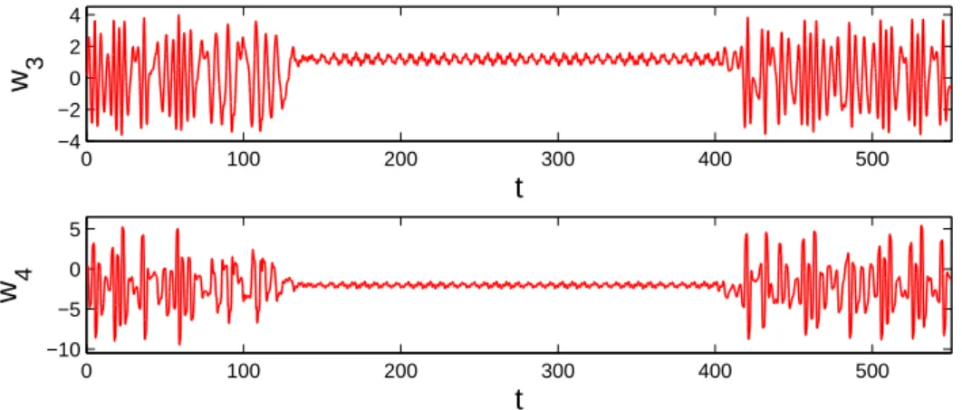
Let us use the OGY control method around the fixed point 2.9/3.9 of the logistic map (5.3) so that λ_j in (5.9) is given by the formula (5.8) withκ⁽ⁱ⁾ ≡ 2.9/3.9. The control mechanism is switched on att=ζ₇₀using the valuesε=0.085 andC=2.6. The OGY control is switched off att =ζ₃₅₀and the Pyragas control is switched off att=ζ₄₀₀. More precisely, we takeλ_j ≡_3.9, C = 2.6 forζ₃₅₀ ≤ t < ζ₄₀₀, and we take λ_j ≡ 3.9,C= 0 forζ₄₀₀ ≤ t ≤ζ₅₅₀. Figure 5.4shows the simulation results for thew₃andw₄coordinates of the control system (5.9) corresponding to the initial data w₁(_0.41) = _0.8, w₂(_0.41) = _0.7, w₃(_0.41) = _0.12, w₄(_0.41) = _{0.013, and} w₅(0.41) = 0.41. It is seen in Figure 5.4 that one of the quasi-periodic solutions of (5.7) is stabilized such that the control becomes dominant approximately att =144 and its effect lasts until t = 400, after which the instability becomes dominant and irregular behavior develops

again. To present a better visuality, the stabilized quasi-periodic solution of (5.7) is shown in Figure5.5 for 200≤ t≤300. Both of the Figures5.4and5.5confirm the presence of infinitely many quasi-periodic motions in the dynamics of (5.7).

0 100 200 300 400 500

−4

−2 0 2 4

t

w 3

0 100 200 300 400 500

−10

−5 0 5

t

w 4

Figure 5.4: Chaos control of system (5.7). We make use of the OGY control method around the fixed point 2.9/3.9 of the logistic map (5.3). The values ε=0.085 andC=2.6 are used in the simulation.

200 210 220 230 240 250 260 270 280 290 300

0.8 1 1.2 1.4 1.6

t

w 3

200 210 220 230 240 250 260 270 280 290 300

−2.5

−2

−1.5

t

w 4

Figure 5.5: The stabilized quasi-periodic solution of system (5.7).

Appendix

For the convenience of the reader, we present and prove a Gronwall–Coppel type inequality (see [10]) result used in this paper.

Theorem A.1. Let a, b, c, andγbe constants such that a≥0, b≥0, c >0,γ>0, and suppose that ϕ(t)∈C([r₁,r₂],R)is a nonnegative function satisfying

ϕ(t)≤a+b

e^{−γ(t−r1)}+e^{−γ(r2−t)} +c

Z _r2

r1

e^−γ|t−s|ϕ(s)ds, t∈ [r₁,r2].