TAMÁSKOCSIS
With the determination of principal parameters of producing and pollution abatement technologies, this paper quantifies abatement and external costs at the social optimum and analyses the dynamic relationship between technological development and the above-mentioned costs. With the partial analysis of parameters, the paper presents the impacts on the level of pollution and external costs of extensive and intensive environmental protection, market demand change and product fees, and not environmental protection oriented technological development. Parametrical cost calculation makes the drawing up of two useful rules of thumb possible in connection with the rate of government in- terventions. Also, the paradox of technological development aiming at intensive environmental protection will become apparent.
1. INTRODUCTION
In connection with environmental protection, a realistic objective for society – accept- ing the neoclassical theory – is not the total termination of all pollution but the forcing back of pollution to a level that ensures the maximization of total social benefits. Ac- cording to this, the pollution level which can be deemed optimal is that where marginal external costs of a certain economic activity deriving from damage done to the envi- ronment equal marginal abatement costs, i.e. a level of pollution from which a move- ment in any direction decreases total social benefits.
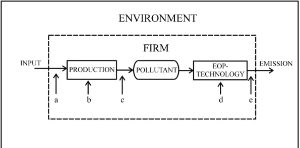
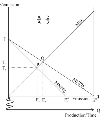
From the point of view of the corporate sector it can be said that the betterment of the state of the environment can be achieved through passive or active environmental meth- ods. The former aims at the reduction of the ambient pollution in the environment with- out reducing emission (at company level such a measure could be the construction of a higher chimney or the dilution of waste water; Fig. 1 – point ‘e’) while active methods actually help in decreasing the amount of pollution emitted during a specific period of time (emission). This paper deals with the latter possibility which may be carried out through two distinct methods. (1) There is a possibility to filter and hold back harmful materials already created during the production process with the help of some kind of
‘end-of-pipe’ (EOP) technology. The introduction and improvement of this method is called extensive technological development (Fig. 1 – point ‘d’). (2) New production technologies and/or inputs can be utilized which result in a smaller amount of harmful materials during the manufacturing process so that the pollutant/unit of production rate actually decreases. A change to such a cleaner technology is called intensive techno- logical development (Fig. 1 – point ‘c’ and ‘a’). Of course, emission can be abated by the reduction of the production level (Fig. 1 – point ‘b’).
While the world of environmentally sound technologies connected to the production process has such a multi-colored nature, today’s environmental economic theories con- tain a certain level of simplification. One of the most important problems concerning this is the merging of different types of pollution abatement costs into one: „The indus-
1 This is the manuscript of a paper which was published in Society and Economy 24 (2002), pp. 69–100.
The author is grateful to the entire staff of the Technology and Environmental Economics Department of the Budapest University of Economic Sciences for an open and friendly atmosphere which made the preparation to this study possible. I am specially indebted to prof. dr. Sándor Kerekes, head of depart- ment, who directed my attention to the unresolved nature of the one polluter - two methods of pollution abatement question and incited me to deal with the problem and to Gyula Zilahy and Michael Mackey who deserve a merit for preparing the English version of this study.
try-wide marginal cost curve (MC) for abatement represents all incremental costs asso- ciated with emission reduction; abatement equipment expenses, costs associated with changes in production processes and/or inputs, and any losses borne by firms and con- sumers due to output modifications” (Milliman–Prince [1989]). This interpretation of abatement costs neglects that (a) while the subsequent abatement of resulting pollution (extensive process) leaves the emission level of profit-maximizing production with no government intervention unchanged, a change in production processes and/or inputs (intensive process) also decreases emissions in real terms; and that (b) although pro- ducer losses originating from the reduction of production are a result of government intervention aiming at the protection of the environment, the size of these is not influ- enced by some separate emission abatement cost function but solely by the total net benefit function of the production process because in this case we are concerned with unrealized earnings resulting from the keeping back of production.
There are theories where among emission abatement costs only the cost of subsequent abatement of already induced pollutants (extensive technique) are taken into account.
That is the right method, but it is often the case that when determining social optimum, they start from the equality of marginal abatement costs and of marginal external costs (e.g. Samuelson–Nordhaus [1985]). All of these unfortunately do not consider that one of the most obvious methods of pollution abatement is the reduction of production lev- els and on the basis of the resulting (quasi) optimum derived with the disregard of this fact such lower emission levels qualify as too expensive. This implicitly suggests the superiority of production over environmental considerations and gives a double push to the increase of GDP/GNP: first through exaggerated production and second through the mitigation of excessive external damages resulting from this higher level of production (Cobb–Halstead–Rowe [1995]). It is nevertheless totally clear that a growth of such nature is expressly harmful and suboptimal at the social level.
These theoretical pitfalls are best avoided by Pearce and Turner (1990) in so far as they strictly distinguish between costs resulting from the keeping back of production and the cleaning of polluting materials resulting from the production process and try to deter- mine the social optimum taking both factors into consideration. Nevertheless, in the end they come to an incorrect conclusion because (1) they use the marginal forgone earnings and marginal abatement cost functions as if these related to total costs, therefore giving a certain unjustified priority to the maintaining of previous levels of production; and – similarly to many of their colleagues – (2) they disregard the specialties deriving from the fact that while marginal net private benefits are a function of the volume of produc- tion the marginal abatement/external cost functions are in close relationship with emis- sions abated/emitted. Although a number of authors mention the importance and nature of the pollutant/unit of production relationship (e.g. Pearce–Turner [1990] p.100; Per- man–Ma–McGilvray [1996], p.202), they do not take the theoretical consequences of these into account. This latter is the most important reason why the effect of intensive procedures – which can be best expressed as a reduction of pollutant/unit of production ratio – has not been demonstrated yet.
2. A GENERAL MODEL OF TECHNOLOGICAL EXTERNALITIES
Our starting point is the analysis of one company with one type of emission for a given period of time. If the industry or a certain group of companies utilizes the same tech- nology then costs and benefits multiplied by the number of participants may give useful aggregate information. During the analysis we assume that all marginal cost and mar-
ginal benefit functions are linear i.e. total cost and total benefit functions can be con- structed with the proper transformations of a parabola.
The production of one company for a given period of time is represented by Q while emissions emitted or abated during the same period shall be denoted with q. These two variables are linked through the linear pollutant/unit of production coefficient according to the relationship2
0
; >
= k
Q
k q . (1)
Now determine the marginal net private benefit (MNPB) curve of the company as a function of production:
0 , )
(Q =b−aQ a b>
MNPB (2)
where b means the market price of the first unit of the product and a means the steep- ness of the function which parameter can be determined on the basis of the relative steepness of the company’s marginal cost and marginal benefit curves.3 As a conse- quence of the definition of the function the maximum amount of total net private bene- fit (TNPB) for a company is
a TNPB b
2
2
max= (3)
Furthermore assume that the producer’s activities have external effects4 in the form of environmental pollution. The marginal external costs (MEC) of this pollution are known by the regulating authority. Let this take the form of a straight line starting from the origin with a positive steepness which shows the size of marginal costs as a function of emissions emitted into the environment:
0 )
(q =eq e>
MEC (4)
where the value of parameter e is in connection with the social impacts of the given emission. The higher its value, the faster social costs arising from external effects in- crease.
During our analysis the company has a technology which is able to subsequently miti- gate a given emission (End-of-pipe-technology = EOP-technology) of which the mar- ginal costs can be determined according to the following formula:
0 )
(q =cq c>
MAC (5)
Furthermore we assume that the EOP-technology given by this cost curve does not be- come scarce over the relevant range. The closer the value of c is to zero the cheaper it is to mitigate a given amount of emission. If we want to exclude the effect of the EOP- technology from the analysis then we will assume that c = +∞ (the MAC curve is verti- cal) i.e. there is no possibility of subsequent mitigation of pollutants created during the
2 All functions, parameters and symbols are summarized in Table III.
3 The MNPB curve is derived from the difference of marginal revenues (MR) and marginal costs (MC):
MNPB(Q)=MR(Q)–MC(Q). If we assume perfect competition the marginal revenue equals the market price [MR(Q)=P], therefore is a horizontal line with zero steepness. Then relationships b=P=MR(Q) and MC(Q)=aQ hold.
4 In our analysis externalities influence the welfare of a third person for which he or she receives no com- pensation and which effect is known but not intentional (see Baumol–Oates [1988], p. 17–18). In the model we do not deal with risks of technologies arising from accidental events.
production process. Remember that abatement costs in MAC consist exclusively of costs arising from the use of EOP type techniques (Fig. 1 – point ‘d’) which – for the sake of separation – should not be taken into account during the calculation of the MNPB curve (MR–MC).
Because the MNPB curve indicates the marginal cost as a function of production while the MAC and MEC curves indicate marginal costs as a function of emissions for our analysis we determine MNPB in relation to emissions:
MNPB q b k
a k q
( )= − 2 (6)
Notice that this relationship gives the marginal benefit formula in relation to production as result only if k = 1. If k ≠ 1 then both the intersection with the vertical axis and the steepness (and thus the intersection with the horizontal axis) of the curve changes while the area under the curve – which indicates the total net private benefit (TNPB) – is un- changed. As k approaches zero (the technology gets cleaner) the curve becomes steeper fitting more tightly to the vertical axis. Emphasizing the necessity of the transformation of the original MNPB(Q) function we will regard the MNPB(q) function as MNPB’ in our study.
Establishing the analytical framework in such a manner we are ready to analyze com- pany pollution abatement behavior. In the following, we assume that the described cost relationships are also characteristic of the whole industry or a well determinable group of companies and therefore there is a possibility to discuss government intervention with social optimum in mind.
3. EXTENSIVE ENVIRONMENTAL PROTECTION
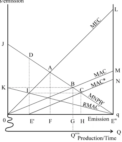
First look at how cost-benefit relationships change at the optimum if the company is forced to mitigate its emissions by some external intervention and has no possibility of using intensive technical solutions (see Fig. 2). On the horizontal axis emissions are indicated in a manner that pollution increases moving away from the origin and Em de- notes the maximal emission relating to the profit-maximizing production level if there is no government intervention. The vertical axis shows the appropriate marginal costs and benefits referring to one unit of emission.
If the company does not have an EOP-technology or the nature of the emission implies that there is no such technique available then the only possibility to mitigate emissions is the keeping back of production. In this case the optimum pollution level is attained at the point where MNPB’=MEC with an external social damage of OAF and forgone earnings of FAEm resulting from the keeping back of production.
Look at the MAC curve now which characterizes the cost relationships of the EOP- technology used by the companies and reflects the amount of mitigated emissions mov- ing away from the origin. If we are to abate the total emission with this technology then we can do so at a cost of OMEm. At the same time, notice that if we are willing to keep back production to Qmin then total social costs decrease from OMEm (fetishized produc- tion) to OBEm. So that the cost of reaching a zero emission state is smallest if we abate G amount of emissions with an EOP-technology while remaining emissions (Em–G) are abated with the keeping back of production.
If our goal is not the total abatement of all emissions and we accept a pollution level of E’ then a parallel shift of MAC to E’ shows the least cost solution: a total EOP-
abatement cost of E’CH and forgone earnings in the value of HCEm resulting from the keeping back of production.
If we consequently deduct the optimal amount of EOP-abatement from the MNPB’
curve in a horizontal direction then we come to the emission demand function of enter- prises. Taking the linear nature of the MNPB’ and MAC curves into account the demand function necessarily takes a linear form which is unambiguously defined by two of its points. In case of an emission demand of Em (when no government intervention is im- plemented), no EOP-procedure will be undertaken because it would unnecessarily in- crease costs and therefore the demand function – similar to the MNPB’ curve – inter- sects the horizontal axis at Em. To determine the intersection with the vertical axis, it is enough to project the intersection of the MNPB’ and MAC curves (point B) onto the cost axis (point K). It can be seen that, pursuant to the derivation of the curve, sections OG and KB are parallel with each other and are of the same size, similarly sections E’H and IC. We will regard the resulting demand function in the followings as real marginal abatement cost (RMAC).
Because RMAC is the demand function for emissions the territory under RMAC from the point Em to the origin shows the minimum pollution abatement cost for companies resulting from the optimum combination of EOP-technology and the keeping back of production. As a consequence, OBEm=OKEm and E’CEm=E’IEm.
Before a parametrical description of the RMAC function let us introduce the so called EOP efficiency index, which is designated by ε. This index can be quantified in the fol- lowing way:
2 2
ck a
ck
= +
ε (7)
Because of constraints made earlier on the values of the parameters, the value of ε moves within the range of 0 < ε ≤ 1 and shows the ratio to which the use of the EOP- technology decreases pollution abatement costs compared to the case when no EOP- technology is implemented – that is, when the only possibility for mitigation is the limi- tation of production.5 According to this, the area of triangle OKEm (Fig. 2) is exactly ε- times the area of OJEm. From the definition of the index, it follows that the no interven- tion case total net private benefit (TNPBmax=OJEm) multiplied by (1–ε) equals the profit of the company(ies) which can also be realized at a zero emission level (KJEm=OJB;
namely a production of Qmin is possible in any case!) and which is exclusively attribut- able to the use of the EOP-technology because otherwise production should be shut down. In the following we refer to this amount as FB (fixed benefit) because with EOP- abatement this is attainable for the company in any case – independently from emission limits:
( )
FB= 1−ε ⋅TNPBmax (8)
5 From the point of view of the introduction of an EOP-technology lower values of the EOP efficiency index (ε) are more favorable (if there is no EOP-technology then c = +∞ and ε = 1 by definition). This is encouraged by a flatter MAC (cheap pollution abatement, low c) and a relatively steeper MNPB’ which is principally the result of a low pollutant/unit of production ratio.
During the (ceteris paribus) course of extensive technological development the value of parameter c de- creases which reduces the value of ε at the same time so that curves MAC and RMAC become flatter while MNPB’ stays unchanged.
The size of company net benefits depending on the emission is shown by the area under the RMAC curve between the vertical axis and the desired level of emission (e.g. quad- rangle OKIE’ in the case of E’ emission).
After introducing the EOP-efficiency index the determination of RMAC becomes sim- ple and takes the following general form:
k q a k q b
RMAC( )=ε −ε 2 (9)
It can be derived from the MNPB’ function the simplest way [see formula (6)] because both its steepness and its intersection with the vertical axis decreases by ε. Because in its above-mentioned form RMAC must be read from ‘the right to the left’ the total abatement cost is given by the following formula:
2
' ( ) 2
)
(
−
=
=
∫
RMAC q dq a b kaqq RTAC
Em
E
ε ( + constant). (10) Now define the size of emission at the social optimum. Notice that this implies the minimization of the sum of the following three different types of costs (Fig. 2): (1) for- gone earnings derived from the keeping back of production (triangle HCEm); (2) the cost of using the EOP-technology (triangle E’CH); and (3) external costs caused to a third party by the polluting character of production (triangle OIE’). As a consequence at the optimum the MEC=MAC=MNPB’ equivalence should hold. But because RMAC has been derived from the MAC=MNPB’ equivalence the social optimum criteria takes the simpler form of MEC=RMAC. In Fig. 2 this is attained exactly at emission level E’
and the minimum total social cost (TSCmin) relating to environmentally polluting pro- duction is represented by the area of triangle OIEm.
4. INTENSIVE ENVIRONMENTAL PROTECTION
Concentrate now on emission mitigation by intensive technological solutions! As al- ready stated in the introductory section, using intensive solutions the pollutant/unit of production decreases which can be achieved through a change of productive technolo- gies or – to a more limited extent – with the utilization of „cleaner” inputs (Fig. 1 – point ‘c’ and ‘a’).6
For the appropriate separation of effects, let us assume for the time being that (1) apart from the pollutant/unit of production coefficient (k) there is no change in the value of any other parameters; and that (2) there is no available EOP-technology for the compa- nies (ε = 1). The effects of intensive technological development can be seen in Fig. 3.
Fig. 3 demonstrates a 40% decline in pollutant/unit of production ratio so that k1/k0 = 0.6 where k1 means the new and k0 the old technology’s pollutant/unit of produc- tion ratio. It can be easily recognized that the size of the emission level relating to the original total net private benefit (Em0) decreased by 40% to Em1, while the area under the curves representing total benefits is unchanged.7 Taking marginal external costs of pro-
6 For example a company may achieve a lower level of sulfur-dioxide emissions with the burning of coal containing smaller quantities of sulfur which is a quite different type of pollution abatement from mitigat- ing the amount of already created sulfur-dioxide. In the former case the pollutant/unit of production de- creases thus we are concerned with intensive environmental protection.
7 In case an EOP-technology is also available the movement of the RMAC curve is similar. The difference is that its intersection with the vertical axis rises at a smaller rate and thus the size of the area under the curve representing maximum total abatement costs gets smaller as well. This is a result of an improve-
duction into account, the abatement cost of E0PEm0 resulting from the keeping back of production at the former E0 optimum decreases to E1QEm1. It can be considered a reduc- tion because as a result of the equality of the areas under the two MNPB’ curves the PQU<Em1UEm0 relationship holds.
But notice that, in the case of the new optimum, the amount of optimal emission has increased (E1>E0) just like the optimal price relating to one unit of emission (T1>T0).
According to this, the total size of socially optimum externality has increased from the former OPE0 to OQE1. In practice this means that if the industry changes to the tech- nology which is significantly better for the environment then society should suffer a bigger external effect and the regulating authority – depending on the method of envi- ronmental regulation (see Milliman–Prince [1989]) – has to ease the emission norm or increase the supply of free marketable permits (E0 → E1) in order to secure a social op- timum or it will also face an increasing demand (E0 → E1) when increasing emission taxes or the price of auctioned marketable permits (T0 → T1). In the following we are going to call this surprising phenomenon – which contradicts all expectations – the paradox of intensive environmental protection. It occurs because the limitation of pro- duction becomes relatively more expensive after a change in technologies: more units of production should be sacrificed to mitigate a unit of emission because the pollut- ant/unit of production index has improved.
At the same time, it should be recognized that if among the given technological circum- stances the emission in question has a smaller external effect (the MEC curve is flatter, see MEC’ in Fig. 3) then the demonstrated paradox effect does not occur. This means that in case of the diffusion of an environmentally sound technique, the pollution to be emitted at the optimum (E0’ → E1’), the price relating to one unit of emission (T0’ → T1’) and the total external cost to be born by society (ORE0’ → OSE1’) decreases which phenomenon fits common sense environmental expectations. Thus the existence and measure of the paradox effect is a function of marginal external costs and marginal abatement costs which latter can be determined on the basis of production technologies.
This field requires a more detailed analysis. But first let us introduce two very useful measures.
5. INDICATORS DESCRIBING THE EXTERNAL EFFECTS OF A TECHNOLOGY
Denote the so called environmental load index by δ, which can be calculated from the relationship
ek2
δ = . (11)
This shows the extent of the external effect of a given technology because e indicates the social effect relating to the given pollutant (the steepness of MEC) while k relates to how much pollutant is caused by one unit of production. This index can take any values above zero.8
ment in the EOP-efficiency index (ε) because if the MAC curve is left unchanged during the development then pollution abatement becomes more and more favorable compared to the keeping back of production because MNPB’ becomes relatively steeper.
8 Lower values of the environmental load index (δ) are more favorable concerning the external effects of a technology. This means that a flat MEC curve (small e) indicates that the specific technology has rela- tively low impacts on the society while a favorable pollutant/unit of production rate (low k) points at the relatively clean nature of production in connection to the specific pollutant. It is easy to see the favorable nature of a small value of this index because the steepness of MEC(Q) is exactly δ.
If we take the environmental load index (which is independent from the cost- relationships of the technology) and add to it parameter a (corrected by the EOP effi- ciency index) then we receive the relative environmental efficiency index of the given technology for the emission in question as a result. This we denote with η:
δ ε
η= a+ . (12)
This index contains information on the effectiveness of production and abatement tech- nologies and the environmental damaging effects of production.9 As a consequence of the definition of the indices, the relationship 0<δ <η holds in all cases.
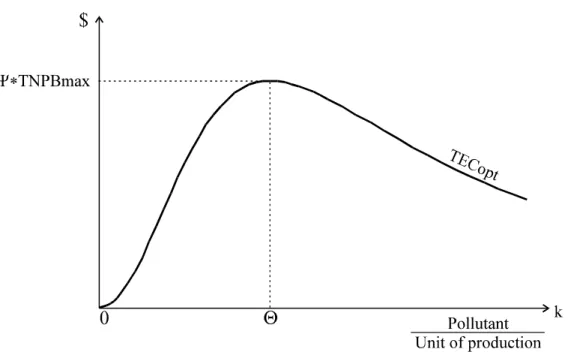
6. THE PARADOX OF INTENSIVE ENVIRONMENTAL PROTECTION In order to determine the exact conditions of the explored paradox effect, we define the socially optimal total external cost (for example the area of the OQE1 triangle when the pollutant/unit of production ratio is k1 as indicated in Fig. 3):
2 2 2
2η ε b δ
TECopt = (13)
Because k, characterizing the effect of intensive environmental protection, has its influ- ence through the value of ε, δ and η, we can analyze the development of total external costs as a function of k. We call the resulting TECopt(k) function the social load function of the technology relating to parameter k. The general form of this function can be seen in Fig. 4. For a given period of time the function shows the optimal extent of external effects to be suffered by the society in the case of different pollutant/unit of production ratios (k) with given technological and external cost relationships (parameters a, c and e). According to this, as intensive technological development produces smaller and smaller pollutant/unit of production ratios (i.e. coming nearer to the origin) the total value of socially optimal external costs gradually increases in the beginning and after the maximum point at Θ decreases dramatically. Θ is the paradox effect threshold relat- ing to parameter k and can be calculated using the following form:
c a e
Θ= a+ (14)
The paradox effect threshold shows that knowing the given production technology, the EOP-technology and the external cost-relationships of the analyzed emission which pollutant/unit of production ratio gives a maximum total external cost at the social op- timum. If the general technical level of the industry has a higher k index than this value then it is probable that we will face a paradox effect during a ceteris paribus intensive technological development if the level of improvement does not reach a certain minimal level.10
9 Lower values of the relative environmental efficiency index (η) are more favorable as far as external effects (e) relative to the efficiency of the producing technology (a) are concerned. First this follows from the features of the environmental load index (δ; footnote 8) and the EOP-efficiency index (ε, footnote 5) described and second from the fact that if parameter a is low (MNPB is flat) this indicates a cheaper pro- duction.
10 In the case of a higher value of the paradox effect threshold (Θ) there is a greater probability that the pollutant/unit of production ratio of the general technical level in reality does not fall in the critical range of k>Θ. This is encouraged by a steep MNPB (high a) and flat MAC and MEC curves (low c and e pa-
Because in reality technological development usually does not occur through a series of infinitely small steps but by leaps with the change of production technology knowing a certain k0>Θ general technical level it can be interesting to analyze the rate of intensive technological development needed – ceteris paribus – in order to avoid the occurrence of the paradox effect. The minimal improvement needed can be calculated with the help of the formula
0 1 0
2
0 0
1 k Θ, k k
k Θ k
k > <
= (15)
where k0 is the pollutant/unit of production ratio of the old technology, k1 is the pollut- ant/unit of production ratio of the new technology and the resulting figure shows to what proportion the new pollutant/unit of production ratio has to decrease compared to the original ratio in order to avoid the paradox effect (thus practically „cutting off” the peak of the social load function). It can be seen that the further k0 lies from the paradox effect threshold the more significant the improvement should be.
The analysis of the maximum point of the social load function gives a very interesting result. It can be proved that this maximum can be calculated with the following for- mula:
a b e c TECopt c
2 4
1 2
(max) ⋅
⋅ +
= (16)
If we divide this amount by the maximum total net private benefit [see formula (3)] we get the maximal social load index of production (Ψ ):
ψ = = ⋅
+ TEC
TNPB
c c e
opt(max) max
1
4 (17)
The maximal social load index of production shows which part of the maximal total net private benefit can account for the total amount of the optimal total external cost deriv- ing from the activity. Because the existence of any EOP-technology only decreases (makes stricter) the value of this index, in the case of non-existence of such a technol- ogy (c = +∞) the Ψmax = 0.25 relationship holds. As a consequence – in case our as- sumption regarding the linearity of marginal costs holds – it can be stated without doubt that if the sum of external costs deriving from emissions relating to the activity of an enterprise (during a given period of time) is greater than one quarter of the maximum total net private benefit relating to the activity then the activity is suboptimal at the so- cial level! The opposite of this statement is not necessarily true, i.e. if external costs are less than one quarter of the total net private benefit than we are not necessarily in the optimum point. But the rule of thumb defined in this way can have a very important role in the identifying and keeping back of activities causing too much external effects.
7. PRODUCT FEE AND CHANGE IN DEMAND
Our model basically concentrates on the cost-benefit relationships of the technology as a function of emissions and thus can be utilized to back up and judge environmental policy decisions relating to emissions. In practice though, taxes and fees are imposed more frequently on products, instead of using the more direct method of emission based rameters). Note that if no EOP-technology is available then it is sufficient to calculate with the formula
e a
Θ= because c = +∞.
intervention. This practice is justified by lower administration and control costs. Be- cause the product fee increases the cost of each product by the same amount its effect can be followed in a decrease of parameter b of the model. This same parameter con- veys the effect of the change in market demand for the product through a change in price, thus Fig. 5 shows the effect of a ceteris paribus decrease in price or product fee introduction.
It can be seen that the introduction of the product fee (or an approximately 60% de- crease in the market price) „pushes” the MNPB’ curve downwards thus significantly decreasing the amount of private total net benefit (OJEm0 → OKEm1). In the case of a price change, the new optimum can be defined on the basis of the RMAC1=MEC rela- tionship (not shown in the figure), but in the case of a pure product fee regulation the possible EOP cleaning technology should not be taken into account i.e. optimization should be carried out only on the basis of the MNPB’ curve. Namely, the company does not optimize in the emission-space but in the product-space, i.e. it attains maximum profits considering the MNPB(Q) = PT (Product Tax) relationship. From this it derives that, in this case, there are no incentives for the company to carry out any emission- mitigation efforts or innovation, thus, looking at direct abatement costs, the product tax can be a quite costly method from a social point of view if we are primarily aiming at emission mitigation objectives.
The optimal value of the product fee from the point of view of regulating emissions can be determined with the appropriate use of the Pigouvian method (1920), i.e. the benefit maximizing production of the company is optimal with respect to external costs can be achieved. Because we have to consider the pollutant/unit of production index and the irrationality of utilization of the EOP-technology when determining the product fee11, its optimal value can be calculated using
δ δ
= + a
PTopt b . (18)
It can be seen that, apart from parameters characterizing the product space, only the environment load index has a role in this equation.
8. NOT ENVIRONMENTAL PROTECTION ORIENTED TECHNOLOGICAL DEVELOPMENT
Before generalizing our model we are going to analyze the case of technical develop- ment which can be followed up in a ceteris paribus decline of parameter a and which does not aim at environmental objectives (Fig. 6). Because now technical development makes the manufacturing and sale of more products possible, the maximum emission (Em0 → Em1) just like the total net private benefit (OJEm0 → OJEm1) increases while the intersection with the vertical axis stays unchanged. This increase in benefits easily off- sets the increase in pollution abatement costs (E0PEm0 → E1QEm1). Concerning the op- timum of external effects12, we can experience a similar effect to the paradox of inten- sive technical development but in this case it is obvious since no environmental con- cerns are involved. Notice also that the higher the steepness of MEC relative to MNPB’
11 Of course even when product fees are implemented companies can be made to use EOP-technologies with the use of other complimentary measures.
12 To simplify Fig. 6 we assume that no EOP-technology exists. The RMAC curve would move similarly only the vertical intersection would also increase to a small extent. This is due to a moderate deterioration in the EOP efficiency index (ε).
(or relative to the RMAC curve in the case of an EOP-technology), the smaller the in- crease in the optimal pollution level because in this case the relative danger posed by the emission does not allow to make excessive concessions to benefits more easily at- tainable with non-environmental technical development at the expense of the social- natural environment.
9. A GENERAL MODEL OF TECHNOLOGY-EVALUATION
Before expressing quantities characterizing the social optimum of production with a few easy to use formulae we introduce a useful index which makes it possible to suc- cinctly express the external effects of a technology. Let us divide the sum of total exter- nal costs and real total abatement costs at the optimum (Total Social Cost, TSC) by the maximum total net private benefit and call this ratio the rate of inevitable external loss of a technology. Denoting this by Ω :
η εδ + =
=
TNPBmax
RTAC
Ω TECopt opt (19)
The rate of inevitable external loss of a technology (taking into account the joint charac- teristics of the analyzed production method and relating EOP-technology) shows what part of the maximum total net private benefit of the technology user is lost inevitably because of the negative external effect of the activity (for a given emission). It is obvi- ous that if there are several technologies available for a given social objective then – assuming that TNPBmax stays unchanged – the technology with a lower Ω must be given priority.13 We have to take care because the Ω value of a technology relates to the social optimum and if we are not producing at this point then the loss rate increases in all cases and – in the case of an inferior production technology (see later) – the ana- lyzed cost/benefit ratio can increase to above 1!
We have arrived to a point where we can quantify the most important parameters of optimal environmental effects of technologies (see Fig. 7). If no EOP-technology exists (ε =1) then [according to formula (8)] FB=0 and we arrive at an unchanged form of the well-known figure (e.g. Pearce–Turner [1990], p. 63) because in this case RMAC=MNPB’. The economic content of each area and its calculation (its size relative to maximum total net private benefit) is contained in Table I. We arrive at the absolute value of damages and benefits if we multiply the values of the table by the value of TNPBmax according to formula (3). In Table II we have summarized the calculation of the most important emission and production levels and the optimal unit of emission tax.
Compared to cases described above – when only the value of a single parameter has been changed at any one time – in reality a change in technology influences the value of all parameters in different directions at the same time. These cases can be handled eas-
13 The rate of inevitable external loss (Ω) describes all important features of the technology from the point of view of external effects, thus its characterization can only be complex. A decline in the value of the index is preferable in accord with the features of the EOP-efficiency index (ε, footnote 5) and the envi- ronmental load index (δ, footnote 8). The fact that the environmental efficiency index, η is in the de- nominator of the expression is seemingly contradicting the explanation in footnote 9, according to which a decrease in η is favorable. But in our case the δ/η rate should be analyzed and this decreases when the environmental load index (δ) is lower relative to the value of parameter a (steepness of the MNPB curve) so that when the technology damages the environment at a lower rate relative to its profitability. This is in accord with our expectations relating to the favorable nature of a low Ω. Also, note that multiplying the maximum total net private benefit (TNPBmax) by (1–Ω) gives the maximum of social net benefit resulting from the use of the technology.
ily with the help of the expressions contained in the tables because, with the determina- tion or estimation of the five key parameters (a, b, c, e, k), required quantities can be determined and analyzed with the aim of either to make the right choice between alter- natives or to analyze general development trends.
10. AN INFERIOR TECHNOLOGY
The tables point at a number of interesting relationships from which the one concerning the ratio of total external costs without intervention (TECmax) requires our special inter- est. If we divide this quantity by the maximum total net private benefit (TNPBmax) then we arrive at an index which characterizes the technology from the point of view of so- cial sustainability (δ/a; Table I, row B+C+D). If this value is larger than 1 for a given technology, which means that the environmental load index (δ ) of the emission in question is higher than the value of parameter a (which indicates the production effi- ciency of the technology), then we call this technology an inferior technology relating to the given emission because its use – with no intervention – results in a larger social damage than the value of its benefits. In this case, even the total withdrawal of profits created during the production process would not be enough to compensate for the social damages and other financial sources should be considered. Such a situation is shown by Fig. 7 in which the intersection of the MNPB’ curve (not RMAC!) with the vertical axis is smaller then the height of the MEC curve at the maximum emission level (Em ).
We can not of course conclude that the use of all inferior technologies should be stopped but this phenomenon inevitably requires intervention. From a social point of view the implementation of an emission (production) level determined on the basis of the MEC=RMAC relationship would be the most favorable but we might have to make a compromise for political reasons. In the case of an inferior technology it could be use- ful to determine the emission (production) level at which private benefits from produc- tion cover external damages. This quantity can be determined with the help of the rela- tionship
a a
Esust bk >
−
+ +
= δ ε δ
ε
η ε ;
) 1
( , (20)
which indicates the socially sustainable emission level for an inferior technology. Note that if no EOP-technology exists then the expression takes the simple form of
bk a
Esust = ε = δ >
η ; 1 and
2 (21)
which is exactly twice the emission level relating to optimal social costs. Thus, if we have pushed down production to the sustainable emission level with the help of some government intervention then we have not yet arrived at the least social cost solution but at least secured that production efforts do not cause a greater damage than the bene- fits arising from them.
11. CONCLUSIONS
The classification of emission mitigating possibilities of companies (extensive/intensive techniques and reduction of production) makes it possible to further refine former envi- ronmental economics approaches. The determination of significant parameters of pro- duction and emission mitigation facilitates the analysis of optimal emission levels and of changes in external costs deriving from the different movements of the real marginal
abatement cost curve. It also helps in differentiating between environmental regulatory means and in evaluating technologies at the company level. These possibilities can mean an appropriate answer to the invitation of Jung, Krutilla and Boyd made at the end of their article on the relationship between industry level technological change and environmental policy (1996) according to which relating environmental economics ap- proaches should become more complex. Knowing the appropriate parameters – with necessary cautiousness – it becomes possible to lay down the foundations of a differen- tiated intervention relating to a given emission because, for example, on the basis of the polluting material content of utilized inputs (e.g. the sulfur content of coal) or of the features of production and EOP-technologies, different types and rates of intervention can mean a lower social cost.
The summary of the model which requires the determination of only five parameters can be found in Table III. The most important constraint of the model is the assumption of linearity and the difficulties experienced during the determination of external costs but consequences reached – at least in their tendencies – are valid an the case of non- linear or estimated external costs14, as well. The procedure drawn up can be extended in a non-linear direction in which case more difficult mathematical instruments will be needed.
The relationship of environmental protection and economic growth has been looked at from a new perspective. In the first place, it has to be seen that the keeping back of pro- duction to a certain extent is more favorable at a social level than subsequent damage mitigation of excessive economic activities even in the case when EOP-technologies are available. At the same time, both extensive and intensive environmental technical de- velopment help increase the optimal level of production but attention has to be given to the fact that on the basis of our model, optimization can be carried out only by one – although usually the most important – type of emission of production. During an envi- ronmentally favorable technical development there are trade-offs, for example end-of- pipe air and water pollution abatement increases the damage caused to the soil through the creation of hazardous wastes, while in the case of change of production technologies often other emissions become dangerous (think of the example of fossil fuel and nuclear power stations). For this reason, there is a need to elaborate models which make it pos- sible to carry out social optimization with the joint involvement of more emissions.
Two important rules of thumb have been identified for environmental policy. According to these, attention has to be paid to the fact that if we are aiming at the social optimum then the total amount of external costs deriving from production should never be greater than one quarter of the maximal total net private benefit with the given technology in the first hand, while on the other, in the case of inferior technologies, there is a need for intervention even if we have to allow – for political or technical reasons – a higher level of production than the optimal. In this case, no intervention means that our production efforts cause more damage than benefits and, for example in developed countries, the continuous decline of more complex indices than GDP15 indicates such processes.
The analysis of intensive environmental protection led to the surprising result that, un- der some circumstances, an environmentally sound development can lead to a higher level of pollution becoming feasible. If we assume a strong relationship between eco-
14 Mainly at industry level it is possible to give interval estimates for some hard to quantify parameters and then we would receive results in the form of intervals as well. Optimization in this case is based on a probabilistic approach.
15 Such indices are for example the Index of Sustainable Economic Welfare (ISEW, Daly–Cobb [1989]) or the Genuin Progress Indicator (GPI, Cobb–Halstead–Rowe [1995]).
nomic development in terms of GDP and the environmental performance of production technologies then it can easily happen that this phenomenon – even though only par- tially because of the optimum assumption and the ceteris paribus analysis – can give an explanation for the empirical relationship identified between the growth of GDP and the emission of certain short term pollutants (environmentally Kuznetz curve). According to this, in spite of environmental protection efforts, an increase in pollution can be ex- perienced parallel to economic growth for some period of time while, over a certain level, a decrease in some types of emissions (e.g. in the case of lead, SO2, dust) can be noticed (e.g. Shafik–Bandyopadhyay [1992]). The cone-shaped curve we can draw up in this way reminds very much of the shape of the social load function relating to inten- sive technological development. In the case of certain emissions (e.g. CO2), an increase can be experienced even in the most developed countries (Holtz-Eakin–Selden [1995]) which can mean that, in the case of these emissions, the general level of technical de- velopment captured by the pollutant/unit of production ratio has not decreased below the paradox effect threshold denoted by Θ (which point may fluctuate as a function of technical parameters). But – taking into account the above-mentioned trade-offs – I dis- agree with the notion that the necessary consequence of this is further economic growth and that the implementation of intensive technical developments is identical to the growth pressure of the economy. These theoretical conclusions are considerably in har- mony with Hilton and Levinson’s empirical results an automotive lead emissions.
In the end, we have to draw attention to the fact that all our theoretical conclusions are valid in the framework of neoclassical economics. The notion of external effects de- scribes the welfare of a third person or persons, thus the approach is basically anthropo- centric. There is an optimal level of pollution which is a function of the society’s indus- trial/economic development and its system of values. The analysis does not concern the right to existence of other living organisms and the description of irreversible processes as a result of environmental pollution. Theoretically, we can take into account a number of damages of this type among external costs, the question is which one to include and to what extent? Another problem is whether damages beyond the social sphere can at all be expressed with the help of such a social category like money and whether the com- plex systems of objectives of companies can be narrowed to just one dimension: profit maximization. By all means, it is probable that the quantification of processes endan- gering the global ecological balance of the Earth and its long time survival would make the marginal external curve steeper up to a point where it becomes perfectly flexible (vertical) making any social level pollution optimization senseless. All these problems though already lead into the realm of ecological economics.
REFERENCES
Baumol, W. J. – Oates, W. E. [1988]: The Theory of Environmental Policy; 2nd ed., Cambridge Univ. Press, Cambridge
Coase, R. H. [1960]: The Problem of Social Cost. Journal of Law and Economics. 3 (October), p. 1-44.
Cobb, C. – Halstead, T. – Rowe, J. [1995]: If the GDP is Up, Why is America Down?
The Atlantic Monthly. October
Daly, H. E. – Cobb, J. B. Jr. [1989]: For the Common Good. Beacon Press, Boston
Hilton, F. G. H. – Levinson, A. [1998]: Factoring the Environmental Kuznets Curve:
Evidence from Automotive Lead Emissions. Journal of Environmental Economics and Management 35. P. 126–141.
Holtz-Eakin, D. – Selden, T. [1995]: Stoking the fires? CO2 emissions and economic growth. Journal of Public Economics 57(1), p. 85–101.
Jung, C. – Krutilla, K. – Boyd, R. [1996]: Incentives for Advanced Pollution Abatement Technology at the Industry Level: An Evaluation of Policy Alternatives. Journal of En- vironmental Economics and Management 30. p. 95-111.
Milliman, S. R. – Prince, R. [1989]: Firm Incentives to Promote Technological Change in Pollution Control. Journal of Environmental Economics and Management 17. p.
247-265.
Pearce, D. – Turner, R. [1990]: Economics of Natural Resources and the Environment.
The John Hopkins University Press, Baltimore
Perman, R. – Ma, Y. – McGilvray, J. [1996]: Natural Resource & Environmental Economics. Longman. London & New York
Pigou, A. C. [1920]: The Economics of Welfare. McGraw-Hill Book Company, New York
Samuelson, P. A. – Nordhaus, W. D. [1985]: Economics. McGraw-Hill. Inc., New York Shafik, N. – Bandyopadhyay, S. [1992]: Economic Growth and environmental quality:
Time series and cross-section evidence. World Bank Policy Research Working Paper
#WPS904. The World Bank, Washington, DC
TABLE I
Calculation of measures characterizing the social optimum of production with the help of technological indices and parameters
QUANTITY (FIG. 7)
ECONOMIC CONTENT RELATIVE SIZE
(to TNPBmax) A+B+C+FB Maximum of total net private benefit without intervention
(TNPBmax) 1
A+B+C Maximum of real total abatement cost (RTACmax)
ε
FB Profit independent from emissions (1−ε)
B+C Total social cost as a result of externality
(TSCopt = TSCmin) Ω
A+FB Maximum of social net benefit (1− Ω)
B
Social optimum of the total external cost (TECopt);
or the minimum amount paid by producer to the damage sufferer (Coase)a
Ω2⋅a δ A+B+FB Total net private benefit at the optimum
(TNPBopt)
1
2
−
Ω
ε C
Total net private benefit not accepted by the society;
or the optimum of abatement costs; or the minimum amount paid by the damage sufferer to the producer (Coase)a
Ω2 1
⋅ε
D Net loss of overproduction
η δ a
2
B+C+D
Total external cost without intervention
(TECmax) δ
a
C+D Externality to be avoided 2
2 ( )
η η δ
a a+
⋅
2B Optimal tax revenue 2⋅Ω2⋅a
δ
2C Optimal emission abatement subsidy ε
2⋅Ω2⋅1
a According to the Coase-theorem there is no need for government intervention relating to the external effect of production if property rights are well defined. As a result of the bidding process between the damage sufferer and the one causing the damage the social optimum is automatically reached.
TABLE II
Calculation of significant emission and production levels and
the optimal unit of emission tax with the help of technological indices and parameters QUAN-
TITY (FIG. 7)
ECONOMIC CONTENT VALUE
WITH AN EOP-TECHNOLOGY (0 < c < +∞ and 0 < ε < 1)
VALUE WITHOUT EOP-TECHNOLOGY
(c = +∞ and ε = 1) Em
Maximum emission with- out intervention (unit of emission)
k b
⋅a k b
⋅a Qm
Maximum production without intervention (unit of production/time)
b a
b a Esust
The level of socially sus- tainable emission (δ >a) (unit of emission)
( )
+ + −
⋅ a
k b δ
ε ε
η ε 1 η
k⋅b 2
Qsust
The level of socially sus- tainable production
(δ >a)(unit of prod./time) ε
( )
η ε ε ε δ
b ck a
1 1
2 + + + 1−
2⋅b η Eopt
The level of emission at the social optimum
(unit of emission) εk⋅ηb
η k⋅b
Qopt
The level of production at the social optimum (unit of production/time)
ε ε
b η ck
1
2 +
b
η Topt
optimal
unit of emission tax k
⋅b
Ω k
⋅b η δ
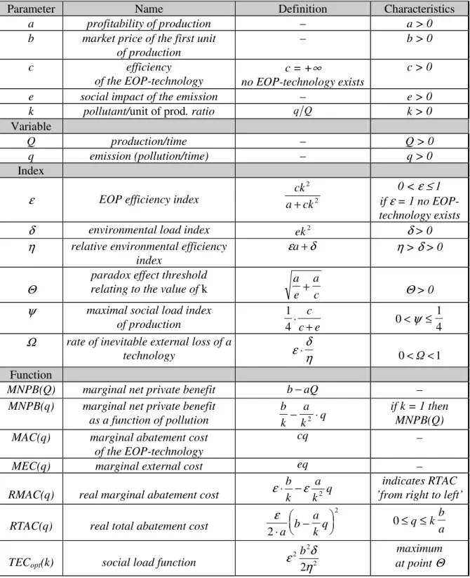
TABLE III
Summary of the elements of the model analyzing the externality of a technology
Parameter Name Definition Characteristics
a profitability of production – a > 0
b market price of the first unit of production
– b > 0
c efficiency
of the EOP-technology
c = +∞
no EOP-technology exists
c > 0
e social impact of the emission – e > 0
k pollutant/unit of prod. ratio q Q k > 0
Variable
Q production/time – Q > 0
q emission (pollution/time) – q > 0
Index
ε EOP efficiency index 2
2
ck a
ck +
0 < ε≤ 1 if ε = 1 no EOP- technology exists
δ environmental load index ek2 δ > 0
η relative environmental efficiency index
δ
εa+ η > δ > 0
Θ
paradox effect threshold
relating to the value of k a e
a
+ c Θ > 0
ψ maximal social load index of production
1 4⋅
+ c
c e 0 1
<ψ ≤ 4 Ω rate of inevitable external loss of a
technology ε δ
⋅η 0<Ω<1 Function
MNPB(Q) marginal net private benefit b−aQ –
MNPB(q) marginal net private benefit as a function of pollution
b k
a k q
− 2 ⋅ if k = 1 then MNPB(Q) MAC(q) marginal abatement cost
of the EOP-technology
cq –
MEC(q) marginal external cost eq –
RMAC(q) real marginal abatement cost q k
a k b
ε 2
ε⋅ − indicates RTAC
’from right to left’
RTAC(q) real total abatement cost ε 2
2
⋅ −
a b a
kq 0≤q≤kb
a
TECopt(k) social load function 2
2 2
2η
ε b δ at point maximum Θ
a: using cleaner inputs resulting a smaller amount of pollutants during the manufactur- ing progress (intensive technique)
b: keeping back of production
c: using new technology resulting a smaller amount of pollutants during the manufac- turing progress (intensive technique)
d: filtering and holding back of pollutants already created during the manufacturing progress (extensive technique)
e: dilution of pollutants before emission (passive method)
FIG. 1. Firm methods influencing emission
FIG. 2. Pollution abatement at the optimum in case of extensive environmental protection
FIG. 3. Pollution abatement at the optimum in case of intensive environmental protection
FIG. 4. Social load function
FIG. 5. Exogenous decrease in demand and the size of the Pigouvian tax
FIG. 6. Not environmental protection oriented technological development
FIG. 7. Measures characterising the social optimum and sustainability
Derivation of Formulae
a) (3) TNPBmax = a b 2
2
from (2): TNPB(Q) = bQ– 2
2Q
a
maximum place: MNPB(Q)=b−aQ= 0
Qmax= a
b (22)
TNPBmax
⇒ =
a b a b a a bb
2 2
2 2 2
=
⋅
−
b) (6) q
k a k q b
MNPB( )= − 2
from (2) and (1)
2 2
) 2
( k
q a k bq q
TNPB = − ⋅
taking its derivative with respect to q we gain (6).
c) (9) RMAC(q)= q k
a k b
ε 2
ε −
from (5) and (6):
B MNP
MAC = ′
k q a k
cq= b − 2
a k c
k b
q 2
= +
Substituting this into MAC (or MNPB’) we receive the intersection with the vertical axis:
c k a kb c
MAC 2
⋅ +
=
On the basis of (7) this can be written in the form of k
ε b which is
the intersection of RMAC(q) with the vertical axis from (22) max ;
a
Q = b from (1) Em =
a kb
qmax = (23)
(by definition this is where it intersects with the horizontal axis).
Let us denote the steepness of the function we are looking for by p.
=
− a
pkb k
εb 0
2 k p=ε a
Thus we gain (9).
d) (10)
∫
′
−
=
=
Em
E
k q b a dq a
q RMAC q
RTAC
2
) 2 ( )
( ε
q E′:=
If the F′
( )
x = f( )
x equation holdsthen
∫
b( )
=( )
−( )
a
a F b F dx x f
from (9)
( )
2 22 q
k q a k q b
F =ε −ε (24)
from (23)
a kb
Em = , thus
max 2
2 2 2 2 2
2 2 2
2 RTAC
a b a b a b a k b k a a kb k F m b
E
q = − = − = =
= ε ε ε ε ε (25)
( )
2 2 22
2 q
k q a k b a q b
F
Fq=Em − =ε −ε +ε From this we gain (10).
e) (8) FB=
(
1−ε)
⋅TNPBmaxBased on (25) and (3)
( )
maxmax
max RTAC 1 TNPB
TNPB − = −ε ⋅
f) (13) 2
2 2
2η ε b δ TECopt =
from (4) and (9)
MEC= RMAC q
k a k eq=εb −ε 2
a ek q bk
ε ε
= 2+
using (12) this is bk EOPT η =
ε (26)
from (4)
2 2 2 2 2
2 1 2 1
η ε b k e TEC
eq TEC
opt = ⋅
=
using (11) we receive (13).
g) (14)
c a e Θ= a+
taking the derivative of (13) with respect to k and looking for the maxi- mum
( )
02 2 2 2
4 + =
−
∂ = c e
e c k a
k TECopt
from this we receive (14) for k.