(2008) pp. 21–30
http://www.ektf.hu/ami
Connection between ordinary multinomials, Fibonacci numbers, Bell polynomials and
discrete uniform distribution ∗
Hacène Belbachir, Sadek Bouroubi, Abdelkader Khelladi
Faculty of Mathematics, University of Sciences and Technology Houari Boumediene (U.S.T.H.B), Algiers, Algeria.
Submitted 8 July 2008; Accepted 16 September 2008
Abstract
Using an explicit computable expression of ordinary multinomials, we establish three remarkable connections, with theq-generalized Fibonacci se- quence, the exponential partial Bell partition polynomials and the density of convolution powers of the discrete uniform distribution. Identities and vari- ous combinatorial relations are derived.
Keywords: Ordinary multinomials, Exponential partial Bell partition poly- nomials, Generalized Fibonacci sequence, Convolution powers of discrete uni- form distribution.
MSC:05A10, 11B39, 11B65, 60C05
1. Introduction
Ordinary multinomials are a natural extension of binomial coefficients, for an appropriate introduction of these numbers see Smith and Hogatt [18], Bollinger [6]
and Andrews and Baxter [2]. These coefficients are defined as follows: Let q>1 and L>0 be integers. For an integera = 0,1, . . . , qL,the ordinary multinomial
L a
q is the coefficient of thea-th term of the following multinomial expansion 1 +x+x2+· · ·+xqL
=X
a>0
L a
q
xa, (1.1)
with La
1= La
(being the usual binomial coefficient) and La
q= 0 fora > qL.
∗Research supported partially by LAID3 Laboratory of USTHB University.
21
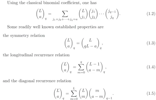
Using the classical binomial coefficient, one has L
a
q
= X
j1+j2+···+jq=a
L j1
j1
j2
· · · jq−1
jq
. (1.2)
Some readily well known established properties are the symmetry relation
L a
q
= L
qL−a
q
, (1.3)
the longitudinal recurrence relation L
a
q
=
q
X
m=0
L−1 a−m
q
, (1.4)
and the diagonal recurrence relation L
a
q
=
L
X
m=0
L m
m a−m
q−1
. (1.5)
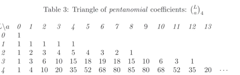
These coefficients, as for usual binomial coefficients, are built trough the Pascal triangle, known as “Generalized Pascal Triangle”, see tables: 1, 2 and 3. One can find the first values of the generalized triangle inSLOANE[17] asA027907forq= 2, A008287forq= 3 andA035343forq= 4.
As an illustration of recurrence relation, we give the triangles of trinomial, quadrinomial and pentanomial coefficients:
Table 1: Triangle oftrinomial coefficients: La
2
L\a 0 1 2 3 4 5 6 7 8 9 10
0 1
1 1 1 1
2 1 2 3 2 1
3 1 3 6 7 6 3 1
4 1 4 10 16 19 16 10 4 1
5 1 5 15 30 45 51 45 30 15 5 1
Table 2: Triangle ofquadrinomial coefficients: La
3
L\a 0 1 2 3 4 5 6 7 8 9 10 11 12
0 1
1 1 1 1 1
2 1 2 3 4 3 2 1
3 1 3 6 10 12 12 10 6 3 1
4 1 4 10 20 31 40 44 40 31 20 10 4 1
Table 3: Triangle ofpentanomial coefficients: La
4
L\a 0 1 2 3 4 5 6 7 8 9 10 11 12 13
0 1
1 1 1 1 1 1
2 1 2 3 4 5 4 3 2 1
3 1 3 6 10 15 18 19 18 15 10 6 3 1
4 1 4 10 20 35 52 68 80 85 80 68 52 35 20 · · ·
Several extensions and commentaries about these numbers have been investi- gated in the literature, for example Brondarenko [7] gives a combinatorial interpre- tation of ordinary multinomials La
q asthe number of different ways of distributing
“a” balls among “L” cells where each cell contains at most “q” balls.
Using this combinatorial argument, one can easily establish the following rela- tion
L a
q
= X
L1+2L2+···+qLq=a
L L1
L−L1
L2
· · ·
L−L1− · · · −Lq−1
Lq
= X
L1+2L2+···+qLq=a
L L1, L2· · ·, Lq
. (1.6)
For a computational view of the relation (1.6) see Bollinger [6]. Andrews and Baxter [2] have considered the q-analog generalization of ordinary multinomials (see also [19] for an exhaustive bibliography). They have defined theq-multinomial coefficients as follows
L a
(p) q
= X
j1+j2+···+jq=a
qPq−l=11(L−jl)jl+1−Pq−l=q−p1 jl+1 L
j1
j1
j2
· · · jq−1
jq
where
L a
= L
a
q
=
(q)L/(q)a(q)L−a if06a6L
0 otherwise
is the usualq-binomial coefficient, and where(q)k=Q∞
m=1(1−qm)/ 1−qk+m , is calledq-series. This definition is motivated by the relation (1.2).
Another extension, the supernomials, has also been considered by Schilling and Warnaar [16]. These coefficients are defined to be the coefficients of xa in the expression ofQN
j=1 1 +x+· · ·+xjLj
A refinement of theq-multinomial coefficient is also considered for the trinomial case by Warnaar [20].
Barry [3] gives a generalized Pascal triangle as n
k
a(n)
:=
k
Y
j=1
a(n−j+ 1)/a(j),
wherea(n)is a suitably chosen sequence of integers.
Kallas [11] and Noe [14] give a generalization of Pascal’s triangle by considering the coefficient of xa in the expression of (a0+a1x+· · ·+aqxq)L.
The main goal of this paper is to give some connections of the ordinary multino- mials with the generalized Fibonacci sequence, the exponential Bell polynomials, and the density of convolution powers of discrete uniform distribution. We will give also some interesting combinatorial identities.
2. A simple expression of ordinary multinomials
If we denotexi the number of balls in a cell, the previous combinatorial inter- pretation given by Brondarenko is equivalent to evaluate the number of solutions of the system
x1+· · ·+xL=a,
06x1, . . . , xL6q. (2.1)
Now, let us consider the system (2.1). Fort∈]−1,1[, we have (see also Comtet [8, Vol. 1, p. 92 (pb 16).])
X
a>0
L a
q
ta= (1 +t+· · ·+tq)L= X
06x1,...,xL6q
tx1+···+xL,
and
(1 +t+· · ·+tq)L= 1−tq+1L
(1−t)−L
=
L
X
j=0
(−1)j L
j
tj(q+1)
X
j>0
j+L−1 L−1
tj
.
By identification, we obtain the following theorem.
Theorem 2.1. The following identity holds
L a
q
=
⌊a/(q+1)⌋
X
j=0
(−1)j L
j
a−j(q+ 1) +L−1 L−1
. (2.2)
This explicit relation seems to be important since in contrast to relations (1.2), (1.3) and (1.5), it allows to compute the ordinary multinomials with one summation symbol.
In 1711, de Moivre (see [13] or [12, 3rd ed. p. 39]) solves the system (2.1) as the right hand side of (2.2).
Corollary 2.2. We have the following identity
⌊n/2⌋
X
j=0
n j
n−j j
=
⌊n/3⌋
X
j=0
(−1)j n
j
2n−3j−1 n−1
.
Proof. It suffices to use relation (6) in Theorem 2.1 for q= 2anda=L=n.
The left hand side of the equality has the following combinatorial meaning. It computes the number of ways to distribute n balls into n boxes with 2 balls at most into each box. Put a ball into each box, then choose j boxes for removing the boxes located in them intoj boxes chosen from the remainingn−j boxes.
3. Generalized Fibonacci sequences
Now, let us consider forq>1, the “multibonacci” sequence(Φ(q)n )n>−q defined by
Φ(q)−q=· · ·= Φ(q)−2= Φ(q)−1= 0, Φ(q)0 = 1,
Φ(q)n = Φ(q)n−1+ Φ(q)n−2+· · ·+ Φ(q)n−q−1 forn>1.
In [4], Belbachir and Bencherif proved that Φ(q−1)n = X
k1+2k2+···+qkq=n
k1+k2+· · ·+kq
k1, k2,· · · , kq
,
and, forn>1
Φ(q−1)n =
⌊n/(q+1)⌋
X
k=0
(−1)k n−k(q−1) n−kq
n−kq k
2n−1−k(q+1),
leading to
X
k1+···+qkq=n
k1+· · ·+kq
k1,· · · , kq
=
⌊n/(q+1)⌋
X
k=0
(−1)kn−k(q−1) n−kq
n−kq k
2n−1−k(q+1).
This is an analogous situation in writing above a multiple summation with one symbol of summation. On the other hand, we establish a connection between the ordinary multinomials and the generalized Fibonacci sequence:
Theorem 3.1. We have the following identity
Φ(q)n =
qm−r
X
l=0
n−l l
q
, (3.1)
wheremis given by the extended euclidean algorithm for division: n=m(q+ 1)−r, 06r6q.
Proof. We have
Φ(q)n = X
k1+2k2+···+(q+1)kq+1=n
k1+k2+· · ·+kq+1
k1, k2,· · ·, kq+1
=X
L>0
X
k1+2k2+···+(q+1)kq+1=n
L k1, k2,· · ·, kq+1
=X
L>0
X
k2+2k3+···+qkq+1=n−L
L
L−k2− · · · −kq+1, k2,· · ·, kq+1
=X
L>0
L n−L
q
=
n
X
L>q+1n
L n−L
q
,
using the fact that La
q = 0fora <0ora > qL
Now consider the unique writing ofngiven by the extended euclidean algorithm for division: n=m(q+ 1)−r,06r < q+ 1then q+1n =m−q+1r ,which gives
Φ(q)n =
qm−r
X
k=0
m+k qm−r−k
q
=
qm−r
X
k=0
m+k (q+ 1)k+r
q
=
qm−r
X
l=0
n−l l
q
.
As an immediate consequence of Theorem 3.1, we obtain the following identities Φ(q)(q+1)m=
qm
X
l=0
(q+ 1)m−l l
q
=
qm
X
k=0
m+k (q+ 1)k
q
,
Φ(q)(q+1)m−1=
qm−1
X
l=0
(q+ 1)m−l−1 l
q
=
qm
X
k=0
m+k (q+ 1)k+ 1
q
, ...
Φ(q)(q+1)m−r=
qm−r
X
l=0
(q+ 1)m−l−r l
q
=
qm
X
k=0
m+k (q+ 1)k+r
q
.
Forq= 1,we find the classical Fibonacci sequence:
F−1= 0, F0= 1, Fn+1=Fn+Fn−1, forn>0.
Thus, we obtain the well known identity Fn =
⌊n/2⌋
X
l=0
n−l l
.
Recently, in [5], the first author and Szalay prove the unimodality of the se- quence uk = n−kk
q associated to generalized Fibonacci numbers. More generally, they establish the unimodality for all rays of generalized Pascal triangles by showing that the sequencewk= m+βkn+αk
q is log-concave, then unimodal.
4. Exponential partial Bell partition polynomials
In this section, we establish a connection of the ordinary multinomials with exponential partial Bell partition polynomials Bn,L(t1, t2, . . .) which are defined (see Comtet [8, p. 144]) as follows
1 L!
X
m>1
tm
m!xm
L
= X
n>L
Bn,Lxn
n!, L= 0,1,2, . . . . (4.1) An exact expression of such polynomials is given by
Bn,L(t1, t2, . . .) = X
k1+2k2+···=n k1+k2+···=L
n!
k1!k2!· · ·(1!)k1(2!)k2· · ·tk11tk22· · ·.
In this expression, the number of variables is finite according tok1+ 2k2+· · ·= n.
Next, we give some particular values ofBn,L: Bn,L(1,1,1, . . .) =
n L
Stirling numbers of second kind, Bn,L(0!,1!,2!, . . .) =
n L
Stirling numbers of first kind, Bn,L(1!,2!,3!, . . .) = n!
L!
n−1 n−L
. (4.2)
In [1], Abbas and Bouroubi give several extended values ofBn,L.
The connection with ordinary multinomials is given by the following result:
Theorem 4.1. We have the following identity
Bn,L(1!,2!, . . . ,(q+ 1)!,0, . . .) = n!
L!
L n−L
q
. (4.3)
Proof. Taking in (4.1)tm=m!for16m6q+ 1and zero otherwise, we obtain x+· · ·+xq+1L
=L! X
n−L>0
Bn,L(1!,2!, . . . ,(q+ 1)!,0, . . .)xn n!,
from which it follows X
a>0
L a
q
xa= X
n−L>0
L!
n!Bn,L(1!,2!, . . . ,(q+ 1)!,0, . . .)xn−L.
Corollary 4.2. Let q>1,L >0 be integers, and a∈ {0,1, . . . , qL}.For q>a, we have the following identity
L a
q
=
L+a−1 a
.
Proof. Using the fact thatBn,L(1!,2!, . . . ,(q+ 1)!,0, . . .) =Bn,L(1!,2!,3!, . . .)for q+ 1 >n−L+ 1, we obtain n−LL
q = n−Ln−1
forq >n−L. We conclude with
a=n−L.
This is simply a combination with repetition permitted (i.e. multi combination).
5. Convolution powers of discrete uniform distribu- tion
This section gives a connection between the ordinary multinomials and the convolution power of the discrete uniform distribution. The right hand side of identity (2.2) is a very well known expression. Indeed for q, L∈N, let us denote byUq⋆L theLthconvolution power of the discrete uniform distribution
Uq := 1
q+ 1(δ0+δ1+· · ·+δq) (δa is the Dirac measure),
then for a∈N(see de Moivre [13] or [10]), with respect to the counting measure, its density is given by
P Uq⋆L=a
= 1
(q+ 1)L
⌊a/(q+1)⌋
X
j=0
(−1)j L
j
a+L−(q+ 1)j−1 L−1
. (5.1)
Combining Theorem 2.1 and relation (5.1), we have the following result:
Corollary 5.1. Using the above notations, we obtain the following identity
P Uq⋆L=a
=
L a
q
(q+ 1)L.
It should be noted that the multinomials may be seen as the number of favorable cases to the realization of the elementary event{a}.
It is easy to show that the distribution ofUq⋆L is symmetric by relation (1.3).
Corollary 5.2. We have the following identities
qL
X
k=0
k L
k
q
= (q+ 1)LqL 2 ,
qL
X
k=0
k2 L
k
q
= (q+ 1)LqL 2
qL
2 +q+ 2 6
,
qL
X
k=0
k3 L
k
q
= (q+ 1)L qL
2
2qL
2 +q+ 2 2
,
More generally, form>1,the following identity holds
qL
X
k=0
km L
k
q
= (q+ 1)L X
i1+i2+···+iL=m
m i1, i2, . . . , iL
ui1ui2· · ·uiL,
whereui is thei-th moment of the random variable Uq.
Proof. It suffices to compute the expectation ofUq⋆L using, first the density distri- bution and second the summation of uniform distributions. It also comes from the application of the generating function of the distribution given by Corollary 5.1.
Acknowledgements. The authors are grateful to Professor Miloud Mihoubi for pointing our attention to Bell polynomials. The authors are also grateful to the referee and would like to thank him/her for comments and suggestions which im- proved the quality of this paper.
References
[1] Abbas, M., Bouroubi, S., On new identities for Bell’s polynomials, Disc. Math., 293 (2005) 5–10.
[2] Andrews, G.E., Baxter, J., Lattice gas generalization of the hard hexagon model IIIq-trinomials coefficients,J. Stat. Phys., 47 (1987) 297–330.
[3] Barry, P., On Integer-sequences-based constructions of generalized Pascal triangles.
Journal of integer sequences, Vol. 9 (2006), Art. 06.2.4.
[4] Belbachir, H., Bencherif, F., Linear recurrent sequences and powers of a square matrix.Integers, 6 (2006), A12, 17 pp.
[5] Belbachir, H., Szalay, L., Unimodal rays in the regular and generalized Pascal triangles,J. of Integer Seq., Vol. 11, Art. 08.2.4. (2008).
[6] Bollinger, R.C., A note on PascalT-triangles, Multinomial coefficients and Pascal Pyramids,The Fibonacci Quarterly, 24 (1986) 140–144.
[7] Brondarenko, B.A., Generalized Pascal triangles and Pyramids, their fractals, graphs and applications, The Fibonacci Association, Santa Clara 1993, Translated from Russian by R.C. Bollinger.
[8] Comtet, L., Analyse combinatoire,Puf, Coll. Sup. Paris, (1970), Vol. 1 & Vol. 2.
[9] Graham, R.L., Knuth, D.E., Patashnik, O., Concrete mathematics, Addison- Wesley, 1994.
[10] Hald, A., A history of mathematical statistics from 1750 to 1930, John Wiley, N.
Y., 1998.
[11] Kallos, G., A generalization of Pascal triangles using powers of base numbers;
Annales mathématiques Blaise Pascal, Vol. 13, no. 1 (2006) 1–15.
[12] de Moivre, A., The doctrine of chances, Third edition 1756 (first ed. 1718 and second ed. 1738), reprinted byChelsea, N. Y., 1967.
[13] de Moivre, A., Miscellanca Analytica de Scrichus et Quadraturis, J. Tomson and J. Watts, London, 1731.
[14] Noe, T.D., On the divisibility of generalized central trinomial coefficients,Journal of Integer sequences, Vol. 9 (2006) Art. 06.2.7.
[15] Philippou, A.N., A note of the Fibonacci sequence of orderkand the Multinomial coefficients,The Fibonacci Quarterly, 21 (1983) 82–86.
[16] Schilling, A., Warnaar, S.O., Supernomial coefficients, Polynomial identities andq-series,The Ramanujan J., 2 (1998) 459–494.
[17] Sloane, N.J.A., The online Encyclopedia of Integer sequences, Published electron- ically athttp://www.research.att.com/~njas/sequences, 2008.
[18] Smith, C., Hogatt, V.E., Generating functions of central values of generalized Pascal triangles,The Fibonacci Quarterly, 17 (1979) 58–67.
[19] Warnaar, S.O., The Andrews-Gordon Identities and q-Multinomial coefficients, Commun. Math. Phys, 184 (1997) 203–232.
[20] Warnaar, S.O., Refinedq-trinomial coefficients and character identities,J. Statist.
Phys., 102 (2001), no. 3–4, 1065–1081.
Hacène Belbachir Sadek Bouroubi Abdelkader Khelladi
USTHB, Faculté de Mathématiques BP 32, El Alia
16111 Bab Ezzouar Alger, Algérie e-mail:
hbelbachir@usthb.dz,hacenebelbachir@gmail.com sbouroubi@usthb.dz,bouroubis@yahoo.fr
akhelladi@usthb.dz,khelladi@wissal.dz