Parametrisation for boundary value problems with transcendental non-linearities
using polynomial interpolation
Dedicated to Professor László Hatvani on the occasion of his 75th birthday
András Rontó
B1, Miklós Rontó
2and Nataliya Shchobak
31Institute of Mathematics, Academy of Sciences of Czech Republic, Branch in Brno, Žižkova 22, 616 62 Brno, Czech Republic
2Institute of Mathematics, University of Miskolc, Miskolc-Egyetemváros, H-3515 Miskolc, Hungary
3Brno University of Technology, Faculty of Business and Management, Kolejní 2906/4, 612 00 Brno
Received 14 January 2018, appeared 26 June 2018 Communicated by Jeff R. L. Webb
Abstract. A constructive technique of analysis involving parametrisation and polyno- mial interpolation is suggested for general non-local problems for ordinary differential systems with locally Lipschitzian transcendental non-linearities. The practical applica- tion of the approach is shown on a numerical example.
Keywords: boundary value problem, transcendental non-linearity, parametrisation, successive approximations, Chebyshev nodes, interpolation
2010 Mathematics Subject Classification: 34B15.
1 Introduction
The present note deals with parametrisation techniques for constructive investigation of boundary value problems and its purpose is to provide a justification of thepolynomialversion of the method suggested in [14].
We consider the non-local boundary value problem
u0(t) = f(t,u(t)), t∈[a,b], (1.1)
φ(u) =γ, (1.2)
whereφ:C([a,b],Rn)→Rn is a non-linear vector functional, f :[a,b]×Rn→Rn is continu- ous in a certain bounded set, and γ∈ Rnis a given vector.
By a solution of the problem (1.1), (1.2) we understand a continuously differentiable vector function with property (1.2) satisfying (1.1) everywhere on[a,b].
BCorresponding author. Email: ronto@math.cas.cz
The idea of our approach (see, e. g., [14,16,17]) is based on the reduction (1.1), (1.2) to a family of simpler auxiliary problems with two-point linear separated conditions ata andb:
u(a) =ξ, u(b) =η, (1.3)
where ξ and η are unknown parameters. By doing so, one can use in the non-local case the techniques adopted to two-point problems [14].
2 Notation and preliminary results
In order to use the reduction to two-point problems (1.1), (1.3), we need some results from [14]. The study of problems (1.1), (1.3) in [14] is based on properties of the iteration sequence {um(·,ξ,η):m≥0}defined as follows:
u0(t,ξ,η):=
1− t−a b−a
ξ+ t−a
b−aη, (2.1)
um(t,ξ,η):=u0(t,ξ,η) +
Z t
a f(s,um−1(s,ξ,η))ds
− t−a b−a
Z b
a f(s,um−1(s,ξ,η))ds, t ∈[a,b], m=1, 2, . . . (2.2) Fix certain closed bounded setsD0,D1 inRnand assume that we are looking for solutions uof problem (1.1), (1.3) with u(a)∈D0andu(b)∈ D1. Put
Ω:={(1−θ)ξ+θη:ξ ∈ D0, η∈ D1, θ∈ [0, 1]} (2.3) and, for any$∈Rn+, define the set
Ω$ :=O$(Ω), (2.4)
where O$(Ω) := Sz∈ΩO$(z) and O$(ξ) := {ξ ∈Rn:|ξ−z| ≤$} for any ξ. Here and be- low, the operations ≤ and |·| are understood componentwise. Set (2.4) is a componentwise
$-neighbourhoodofΩ.
Introduce some notation. Given a domainD⊂ Rn, we write f ∈LipK(D)ifKis an n×n matrix with non-negative entries and the inequality
|f(t,u)− f(t,v)| ≤K|u−v| (2.5) holds for all{u,v} ⊂Dandt ∈[a,b]. We also put
δ[a,b],D(f):= sup
(t,x)∈[a,b]×D
f(t,x)− inf
(t,x)∈[a,b]×Df(t,x). (2.6) The computation of the greatest and least lower bounds for vector functions is understood in the componentwise sense.
The following statement is a combination of Proposition 1 and Theorem 3 from [14].
Theorem 2.1([14]). Let there exist a non-negative vector$satisfying the inequality
$≥ b−a
4 δ[a,b],Ω$(f). (2.7)
Assume, furthermore, that there exists a non-negative matrix K such that r(K)< 10
3(b−a) (2.8)
and f ∈LipK(Ω$). Then, for all fixed(ξ,η)∈D0×D1:
1. For every m, the function um(·,ξ,η)satisfies the two-point separated boundary conditions(1.3) and
{um(t,ξ,η):t ∈[a,b]} ⊂Ω$. 2. The limit
u∞(t,ξ,η) = lim
m→∞um(t,ξ,η) (2.9)
exists uniformly in t∈[a,b]. The function u∞(·,ξ,η)satisfies the two-point conditions(1.3).
3. The function u∞(·,ξ,η)is a unique solution of the integral equation u(t) =ξ+
Z t
a f(s,u(s))ds− t−a b−a
Z b
a f(s,u(s))ds+ t−a
b−a(η−ξ), t∈ [a,b], (2.10) or, equivalently, of the Cauchy problem
u0(t) = f(t,u(t)) + 1
b−a∆(ξ,η), t∈[a,b], u(a) =ξ,
(2.11)
where∆:D0×D1→Rnis a mapping given by the formula
∆(ξ,η):=η−ξ−
Z b
a f(s,u∞(s,ξ,η))ds. (2.12) 4. The following error estimate holds:
|u∞(t,ξ,η)−um(t,ξ,η)| ≤ 10
9 α1(t)Km∗ (1n−K∗)−1δ[a,b],Ω$(f), (2.13) for any t ∈[a,b]and m≥0, where
K∗ := 3
10(b−a)K (2.14)
and
α1(t):=2(t−a)
1− t−a b−a
, t ∈[a,b]. (2.15)
In (2.13) and everywhere below, the symbol 1nstands for the unit matrix of dimension n.
Theorem 2.2([14, Proposition 8]). Under the assumption of Theorem2.1, the function u∞(·,ξ,η): [a,b]×D0×D1 → Rn defined by(2.9) is a solution of problem (1.1),(1.2) if and only if the pair of vectors (ξ,η) satisfies the system of2n equations
∆(ξ,η) =0, (2.16)
φ(u∞(·,ξ,η)) =γ, (2.17)
where∆is given by(2.12).
Equations (2.16), (2.17) are usually referred to asdeterminingequations because their roots determine solutions of the original problem. This system, in fact, determines all possible solutions of the original boundary value problem the graphs of which are contained in the region under consideration.
Theorem 2.3([14, Theorem 9]). Let f ∈ LipK(Ω$)with a certain$satisfying(2.7)and K such that (2.8)holds. Then:
1. if there exists a pair of vectors (ξ,η) ∈ D0×D1 satisfying(2.16), (2.17), then the non-local problem(1.1),(1.2)has a solution u(·)such that
{u(t):t∈ [a,b]} ⊂Ω$ (2.18) and u(a) =ξ,u(b) =η;
2. if problem (1.1), (1.2) has a solution u(·) such that (2.18) holds and u(a) ∈ D0, u(b) ∈ D1, then the pair(u(a),u(b))is a solution of system(2.16),(2.17).
The solvability of the determining system (2.16), (2.17) can be analysed by using its mth approximate version
η−ξ−
Z b
a f(s,um(s,ξ,η))ds=0, (2.19)
φ(um(·,ξ,η)) =γ, (2.20)
wheremis fixed, similarly to [10,12,13,15]. Equations (2.19), (2.20), in contrast to (2.16), (2.17), involve only terms which are obtained in a finite number of steps.
The explicit computation of functions (2.2) (and, as a consequence of this, the construc- tion of equations (2.19), (2.20)) may be difficult or impossible if the expression for f involves complicated non-linearities with respect to the space variable, which causes problems with symbolic integration. In order to facilitate the computation ofum(·,ξ,η),m≥0, one can use a polynomialversion of the iterative scheme (2.2), in which the results of iteration are replaced by suitable interpolation polynomials before passing to the next step. This scheme is described below.
3 Some results from interpolation theory
Recall some results of the theory of approximations [2,3,6]. In a similar situation, we have used these facts in [11].
Denote by Pq a set of all polynomials of degree not higher than q, q ≥ 1, on [a,b]. For any continuous function y : [a,b] → R, there exists a unique polynomial p∗q ∈ Pq, for which maxt∈[a,b]|y(t)−p∗q(t)|= Eq(y), where
Eq(y):= inf
p∈Pqmax
t∈[a,b]|y(t)−p(t)|. (3.1) This p∗q is the polynomial of thebest uniform approximationof yinPq and the numberEq(y)is called theerror of the best uniform approximation.
For a given continuous functiony :[a,b] → Rand a natural numberq, denote by Lqy the Lagrange interpolation polynomial of degreeqsuch that
(Lqy)(ti) =y(ti), i=1, 2, . . . ,q+1, (3.2) where
ti = b−a
2 cos(2i−1)π
2(q+1) + a+b
2 , i=1, 2, . . . ,q+1, (3.3) are the Chebyshev nodes translated from(−1, 1)to the interval(a,b)(see, e. g., [7]).
Proposition 3.1([7, p. 18]). For any q≥1and a continuous function y:[a,b]→R, the correspond- ing interpolation polynomial(3.2)constructed with the Chebyshev nodes(3.3)admits the estimate
y(t)−(Lqy)(t) ≤ 2
πlnq+1
Eq(y), t∈ [a,b]. (3.4) Recall that themodulus of continuity[5, p. 116] of a continuous functiony:[a,b]→Ris the functionδ7→ ω(y;δ), where
ω(y;δ):=sup{|y(t)−y(s)|:{t,s} ⊂[a,b], |t−s| ≤δ} (3.5) for all positive δ. Note that ω(y;·) is a continuous non-decreasing function on (0,∞). A functionyis uniformly continuous if and only if limδ→0ω(y;δ) =0 [5, p. 131].
Proposition 3.2 (Jackson’s theorem; [6, p. 22]). If y∈C([a,b],R),q≥1,then Eq(y)≤6ω
y;b−a 2q
. (3.6)
A functiony : [a,b] →R is said to satisfy the Dini–Lipschitz condition(see, e. g., [3, p. 50]) if its modulus of continuity has the property
lim
δ→0ω(y;δ)lnδ=0.
It follows from (3.6) that
qlim→∞Eq(y)lnq=0 (3.7)
for any y satisfying the Dini–Lipschitz condition. In view of (3.4), equality (3.7) ensures the uniform convergence of Lagrange interpolation polynomials at Chebyshev nodes for this class of functions. In particular, everyα-Hölder continuous function[a,b]→Rwithα>0 satisfies the Dini–Lipschitz condition.
4 Polynomial successive approximations
Rewrite (2.2) in the form
um(t,ξ,η) =u0(t,ξ,η) + (ΛNfum−1(·,ξ,η)])(t), t∈ [a,b], m=1, 2, . . . , (4.1) whereΛis the linear operator in the space of continuous functions defined by the formula
(Λy) (t):=
Z t
a y(s)ds− t−a b−a
Z b
a y(s)ds, t∈[a,b], (4.2) and Nf is the Nemytskii operator generated by the non-linearity from (1.1),
(Nfy) (t):= f(t,y(t)), t∈ [a,b], (4.3) for any continuousy :[a,b]→Rn.
Fix a natural numberqand extend the notation Lqyto vector functions by putting
Lqy:=col(Lqy1,Lqy2, . . . ,Lqyn) (4.4)
for any continuousy:[a,b]→Rn. In (4.4),Lqyi is theqth degree interpolation polynomial for yi at the Chebyshev nodes (3.3). By analogy to (4.4), put
Eqy =col(Eqy1,Eqy2, . . . ,Eqyn). (4.5) IfD⊂Rnis a closed domain and f :[a,b]×D→Rn, put
lq,D(f):= 2
πlnq+1
sup
p∈Pq+1,D
Eq(Nfp), (4.6)
where
Pq,D :=u:u∈ Pqn, u([a,b])⊂ D (4.7) with Pqn := Pq× · · · × Pq. The second multiplier in (4.6) is the least upper bound of errors of best uniform approximations of the functions obtained by substitution into the right-hand side of equation (1.1) of vector polynomials of degree≤q+1 with values in D.
Introduce now a modified iteration process keeping formula (2.1) foru0(·,ξ,η):
vq0(·,ξ,η):= u0(·,ξ,η) (4.8)
and replacing (4.1) by the formula
vqm(t,ξ,η):= u0(t,ξ,η) + (ΛLqNfvqm−1(·,ξ,η))(t), t ∈[a,b], m=1, 2, . . . (4.9) For any q ≥ 1, formula (4.9) defines a vector polynomial vqm(·,ξ,η) of degree ≤ q+1 (in particular, all these functions are continuously differentiable), which, moreover, satisfies the two-point boundary conditions (1.3). The coefficients of the interpolation polynomials depend on the parametersξ andη.
Similarly to (4.1), functions (4.9) can also be used to study the auxiliary problems (1.1), (1.3).
Let Hkβ, where k ∈ Rn+, ki ≥ 0, 0 < βi ≤ 1, i = 1, 2, . . . ,n, be the set of vector functions y:[a,b]→Rnsatisfying the Hölder conditions
|yi(t)−yi(s)| ≤ki|t−s|βi (4.10) for all{t,s} ⊂[a,b],i=1, 2, . . . ,n. Now we can state the “polynomial” version of Theorem2.1.
Theorem 4.1. Let there exist a non-negative vector$such that
$≥ b−a
4 δ[a,b],Ω$(f) +2lq,Ω$(f) (4.11) and f ∈LipK(Ω$)with a certain matrix K satisfying(2.8). Furthermore, let there exist vectors c and βwith ci ≥0,0< βi ≤1, i=1, 2, . . . ,n, such that
f(·,ξ)∈ Hcβ (4.12)
for all fixedξ ∈ Ω$. Then, for all fixed(ξ,η)∈D0×D1:
1. For any m ≥ 0, q ≥ 1, the function vqm(·,ξ,η)is a vector polynomial of degree q+1having values inΩ$ and satisfying the two-point conditions(1.3).
2. The limits
vq∞(·,ξ,η):= lim
m→∞vqm(·,ξ,η), v∞(·,ξ,η):= lim
q→∞vq∞(·,ξ,η) (4.13) exist uniformly on[a,b]. Functions(4.13)satisfy conditions(1.3).
3. The estimate
u∞(t,ξ,η)−vqm(·,ξ,η)≤ 10
9 α1(t)Km∗ (1n−K∗)−1 δ[a,b],Ω
$(f) +lq,Ω$(f) (4.14) holds for any t∈[a,b], m≥0, q≥1, where K∗andα1 are given by(2.14),(2.15).
The proof of this theorem is given in Section5.1. Note thatv∞coincides withu∞appearing in Theorems2.1and2.2.
Similarly to (2.19), (2.20), in order to study the solvability of the determining system (2.16), (2.17), one can use itsmth approximate polynomial version
η−ξ =
Z b
a
(LqNfvqm(·,ξ,η))(s)ds, (4.15)
φ(vqm(·,ξ,η)) =γ, (4.16)
which can be regarded as an approximate version of (2.19), (2.20). If(ξˆ, ˆη)is a root of (4.15), (4.16) in a particular region, then the function
Umq(t):=vqm t, ˆξ, ˆη
, t ∈[a,b], (4.17)
provides themthpolynomial approximationto a solution of the original problem with the corre- sponding localisation of initial data. Of course, system (2.19), (2.20) may have multiple roots;
in such cases, these roots determine different solutions.
It should be noted that, under conditions of Theorem4.1, the function Nfvqm−1(·,ξ,η))ap- pearing in (4.9) always satisfies the Dini–Lipschitz condition and, therefore, the corresponding interpolation polynomials at Chebyshev nodes uniformly converge to it asqgrows to∞. This follows from Lemma5.1of the next section.
Condition (4.11) on$assumed in Theorem4.1is stronger than (2.7) of Theorem2.1due to the presence of an additional positive term on the right-hand side. A stronger version of (2.7) is needed in order to ensure that the values of iterations do not escape from the set where the Lipschitz condition on f is assumed, for which purpose (2.7) is sufficient in the case of iterations (2.1), (2.2).
The value Eq(Nfp), where p ∈ Pq+1, appearing in (4.6) essentially depends on the char- acter of the non-linearity f. In particular, if f is linear, then Eq(Nfp)is the error of the best uniform approximation of a polynomial of degree≤q+1 by polynomials of degree ≤q.
In spite of the presence of an additional expression in (4.11), for which the theorem does not provide explicit estimates, one may however say that, technically, it is (2.7) that plays the most important role here because the extra term is due to the polynomial approximation, the quality of which grows with q. One can treat this in a different way as follows. Instead of assuming condition (4.11), let us suppose that there exists a non-negative vector$such that
$ ≥ b−a
4 δ[a,b],Ω$(f) +r
(4.18)
with a certain strictly positive vectorr. Put
w0(·,ξ,η):= u0(·,ξ,η), (4.19)
wm(t,ξ,η):= u0(t,ξ,η) + (ΛLqmNfwm−1(·,ξ,η))(t), t∈ [a,b], m=1, 2, . . . (4.20) where{qm : m≥1} ⊂N; the choice of this sequence will be discussed below. The condition (2.8) on the maximal in modulus eigenvalue of the Lipschitz matrix K for f in (1.1) is left intact.
Repeating almost word for word the argument from the proof of Theorem 4.1 (see Sec- tion5.1), we find that the sequence {wm(·,ξ,η) : m ≥ 0} defined according to (4.19), (4.20) converges to the same limit as{um(·,ξ,η):m≥0}given by (4.1) provided that
sup
ξ∈D0,η∈D1
sup
m≥1
2
πlnqm+1
Eqm(Nfwqmm−1(·,ξ,η))≤ 1
2r, (4.21)
wherer is the vector appearing in (4.18). Although (4.21) involves the members of sequence (4.19), (4.20), other assumptions on f (namely, (4.12) and the Lipschitz condition in the space variable) and Jackson’s theorem (Proposition3.2) guarantee that, given any value ofrin (4.18), the corresponding condition (4.21) can always be satisfied by choosingq1,q2, . . . appropriately.
This means that the following is true.
Proposition 4.2. Under conditions (2.8), (4.12), and(4.18), sequence (4.19), (4.20) uniformly con- verges provided that qm is chosen large enough at every step m.
In that case, sequence (4.19), (4.20) will serve the same purpose as sequence (4.8), (4.9) under the assumptions of Theorem4.1.
The argument above relies on the knowledge of smallness of the related term appearing on the left-hand side of (4.21). It is however natural to expect that such quantities should diminish if the number of nodes gets larger. To see this, let us now assume conditions somewhat stronger than those of Theorem4.1.
Assume that, instead of (2.8), the matrixK appearing in the inclusion f ∈LipK(Ω$)satis- fies the condition
r(K)< 2
b−a. (4.22)
Theorem 4.3. Let there exist a non-negative vector$and positive vector r such that(4.18)holds and f ∈LipK(Ω$)with K satisfying(4.22). Assume that f(·,ξ)is Lipschitzian with some constant vector c for all fixed ξ ∈ Ω$. Then the iteration process (4.19), (4.20) can be made convergent by choosing qm =q, r=1, 2, . . ., with q sufficiently large.
In other words, under conditions of Theorem4.3, the iteration process (4.19), (4.20) reduces to (4.8), (4.9) withqlarge enough.
5 Proofs
5.1 Proof of Theorem4.1
We shall use several auxiliary statements formulated below.
Lemma 5.1. Let D ⊂ Rn and f : [a,b]×D → Rn be a function satisfying condition (4.12) on D with certain vectors c and β = (βi)ni=1,0< βi ≤ 1, i= 1, 2, . . . ,n. Let f ∈ LipK(D)with a certain n×n matrix K with non-negative entries. If u ∈ Hcβ˜˜ with β˜ = (β˜i)in=1,0< β˜i ≤1, i= 1, 2, . . . ,n, then
Nfu∈ HKµc˜+c, (5.1)
whereµ:=min{β, ˜β}.
Proof. Assume thatu∈ Hcβ˜˜ and the values ofu lie inD. For the sake of brevity, introduce the notation tβ := col(tβ1,tβ2, . . . ,tβn) for any t ∈ [a,b]. Using (4.12) and the Lipschitz condition for f, we obtain
(Nfu) (t)−(Nfu)(s) =|f(t,u(t))−f(t,u(s)) + f(t,u(s))− f(s,u(s))|
≤K|u(t)−u(s)|+c|t−s|β
≤Kc˜|t−s|β˜+c|t−s|β
≤(Kc˜+c)|t−s|µ
with µ = min{β, ˜β}, i. e., the function Nfu satisfies a condition of form (4.10), which proves relation (5.1).
Let the functionsαm :[a,b]→R+,m≥0, be defined by the recurrence relation
α0(t):=1, (5.2)
αm+1(t):=
1− t−a b−a
Z t
a
αm(s)ds+ t−a b−a
Z b
t
αm(s)ds, m=0, 1, 2, . . . (5.3) For m=0, formula (5.3) reduces to (2.15).
Lemma 5.2([8, Lemma 3]). For any continuous function y:[a,b]→R, the estimate
Z t
a
y(τ)− 1 b−a
Z b
a y(s)ds dτ
≤ 1
2α1(t)max
s∈[a,b] f(s)− min
s∈[a,b]f(s), t∈ [a,b], (5.4) holds, whereα1(·)is given by(2.15).
Lemma 5.3([9, Lemma 3.16]). The following estimates hold for all t∈ [a,b]: αm+1(t)≤ 10
9
3(b−a) 10
m
α1(t), m≥0, αm+1(t)≤ 3
10(b−a)αm(t), m≥2.
(5.5)
Let us now turn to theproof of Theorem4.1. Fixξ ∈ D0,η∈ D1, q≥1, and put
yqm := Nfvqm(·,ξ,η) (5.6) form≥0. We need to show that
{vqm(t,ξ,η):t∈ [a,b]} ⊂Ω$ (5.7) for any m. Obviously, (5.7) holds ifm=0.
Form≥1, in view of (2.6), (4.2) and (5.6), Lemma5.2yields the componentwise estimates
|(Λyqm)(t)| ≤ 1
2α1(t)max
s∈[a,b]yqm(s)− min
s∈[a,b]yqm(s)
= 1
2α1(t)max
s∈[a,b]f(s,vqm(s,ξ,η))− min
s∈[a,b] f(s,vqm(·,ξ,η))
≤ 1
2α1(t)δ[a,b],Ω$(f)
≤ 1
4(b−a)δ[a,b],Ω
$(f) (5.8)
for allt∈ [a,b]. In (5.8), we have used the equality max
t∈[a,b]α1(t) = 1
2(b−a) (5.9)
which follows directly from (2.15). Furthermore, using relations (5.4), (5.9) and estimate (3.4) of Proposition3.1, we obtain
|(Λ(Lqyqm−1−yqm−1))(t)| ≤ 1
2α1(t)max
s∈[a,b]
(Lqyqm−1(s)−yqm−1(s))−min
s∈[a,b](Lqyqm−1(s)−yqm−1(s))
≤α1(t)max
s∈[a,b]
|Lqyqm−1(s)−yqm−1(s)|
≤ 1
2(b−a) 2
π lnq+1
Eq(yqm−1). (5.10)
Combining (5.8) with (5.10) and recalling (4.9), we find
vqm(t,ξ,η)−v0q(t,ξ,η)= (ΛLqyqm−1)(t)
= (Λyqm−1)(t) + (Λ(Lqyqm−1−yqm−1))(t)
≤ 1
4(b−a)
δ[a,b],Ω$(f) +2 2
πlnq+1
Eq(yqm−1)
. (5.11) Form=1, (5.11) and condition (4.11) yield
vq1(t,ξ,η)−vq0(t,ξ,η) ≤ 1
4(b−a)
δ[a,b],Ω$(f) +2 2
πlnq+1
Eq(Nfu0(·,ξ,η))
≤ 1
4(b−a)
δ[a,b],Ω$(f) +2lq,Ω$(f)
≤$,
which, by virtue of (2.4), shows that (5.7) holds withm =1. Arguing by induction, we show that (5.7) holds for any m. The values of every function of sequence (4.9) are thus contained inΩ$. Using the Lipschitz condition on f and Proposition3.1, we get
|(Nfum(·,ξ,η))(t)−(LqNfvqm(·,ξ,η))(t)|
≤ |(Nfum(·,ξ,η))(t)−(Nfvqm(·,ξ,η))(t)|+|(Nfvqm(·,ξ,η))(t)−(LqNfvqm(·,ξ,η))(t)|
≤K|um(t,ξ,η)−vqm(t,ξ,η)|+ 2
πlnq+1
Eq(Nfvqm(·,ξ,η)) (5.12) for alltandm.
Let us put
(My) (t):=
1− t−a b−a
Z t
a y(s)ds+ t−a b−a
Z b
t y(s)ds, t ∈[a,b], (5.13) for any continuous vector functiony. Then, according to (4.1), (4.9), (4.6), and (5.12), we obtain
|um(t,ξ,η)−vqm(t,ξ,η)|= |(Λ[Nfum−1(·,ξ,η)−LqNfvqm−1(·,ξ,η)])(t)|
≤ (M|Nfum−1(·,ξ,η)−LqNfvqm−1(·,ξ,η)|)(t)
≤ (M K|um−1(·,ξ,η)−vqm−1(·,ξ,η)|)(t) +
2
πlnq+1
Eq(Nfvqm(·,ξ,η))(Me)(t)
≤ (M K|um−1(·,ξ,η)−vqm−1(·,ξ,η)|)(t) +lq,Ω$(f) (Me)(t) fort ∈[a,b],m≥1, where e=col(1, 1, . . . , 1). In particular,
|u1(t,ξ,η)−vq1(t,ξ,η)| ≤lq,Ω$(f) (Me)(t)
=lq,Ω$(f)α1(t),
|u2(t,ξ,η)−vq1(t,ξ,η)| ≤(M K|u1(·,ξ,η)−vq1(·,ξ,η)|)(t) +lq,Ω$(f) (Me)(t)
≤K(Mlq,Ω$α1e)(t) +lq,Ω$(f)α1(t)
= (Kα2(t) +1nα1(t))lq,Ω$(f). Arguing by induction, we obtain
um(t,ξ,η)−vqm(t,ξ,η)≤ (αm(t)Km−1+αm−1(t)Km−2+· · ·+1nα1(t))lq,Ω$(f), whereαk,k=1, 2, . . . , are given by (5.2), (5.3). Estimate (5.5) of Lemma5.3now yields
um(t,ξ,η)−vqm(t,ξ,η)≤ 10
9 [1n+K∗+K2∗+. . .K∗m−1]α1(t)lq,Ω$(f) with K∗ as in (2.14), whence, due to assumption (2.8),
um(t,ξ,η)−vqm(t,ξ,η) ≤ 10
9 (1n−K∗)−1α1(t)lq,Ω$(f). (5.14) Using (5.14) and estimate (2.13) of Theorem 2.1, we get
u∞(t,ξ,η)−vqm(t,ξ,η)≤ |(u∞(t,ξ,η)−um(t,ξ,η))|+|(um(t,ξ,η)−vqm(t,ξ,η))|
≤ 10
9 α1(t)Km∗ (1n−K∗)−1δ[a,b],Ω$(f) + 10
9 (1n−K∗)−1α1(t)lq,Ω$(f)
= 10
9 α1(t)Km∗(1n−K∗)−1(δ[a,b],Ω$(f) +lq,Ω$(f)), (5.15) whereu∞(·,ξ,η)is a limit function (2.9) of sequence (2.2) (the limit exists by Theorem2.1). In view of (2.8) and (2.14), estimate (5.15) shows that sequence (4.8), (4.9) converges to the same limit.
5.2 Proof of Theorem4.3
We shall use the following Ostrowski inequality [4] for Lipschitz continuous functions [1].
Lemma 5.4([1]). If y: [a,b]→R, y∈ H1c, then
y(t)− 1 b−a
Z b
a y(s)ds
≤ 1
4+
t−12(a+b) b−a
2
c(b−a) (5.16) for all t∈[a,b].
If y ∈ H1c, y : [a,b] → Rn, then c in (5.16) is a vector and the inequality is understood componentwise. Recall that Hc1 is the class of functions y satisfying (4.10) with ki = 1, i = 1, 2, . . . ,n, i. e.,yis Lipschitzian with the vectorc.
In view of the observation made after the formulation of Theorem 4.3, we shall consider sequence (4.8), (4.9).
Fixξ ∈ D0andη∈D1 and writevqm(t) =vqm(t,ξ,η)for the sake of brevity. Let us put cqm := max
t∈[a,b]|v˙qm(t)|, m≥0, q≥1, (5.17) where ˙= d/dt. In other words, cqm is the Lipschitz constant of the polynomial vqm (we know from (4.9) thatvqmis a polynomial of degree≤q+1, i. e.,vqm ∈ Pq+1). Thus,
vqm ∈ H1cq
m. (5.18)
According to (4.2), (4.9), we have
˙
vqm−1(t) =u˙0(t) + (LqNfvqm−2)(t)− 1 b−a
Z b
a
(LqNfvqm−2)(s)ds. (5.19) Since, by (2.1),
u˙0(t) = 1
b−a(η−ξ), (5.20)
it follows from (5.19) and Lemma5.4that
|v˙qm−1(t)| ≤ 1
b−a|η−ξ|+ 1 4+
t− 12(a+b) b−a
2!
(b−a)λqm−2, (5.21) whereλqm−2 is the Lipschitz constant (actually, vector) of the vector function Nfvqm−2.
By assumption, f satisfies condition (4.12) with β = 1. Therefore, by virtue of equality (5.17) and Lemma5.1,
Nfvqm−2∈ HKc1 q
m−2+c (5.22)
and, hence,
λqm−2≤ Kcqm−2+c. (5.23)
It is easy to check that
tmax∈[a,b](2t−a−b)2 = (b−a)2
and, therefore, combining (5.21) and (5.23), we obtain
|v˙qm−1(t)| ≤ 1
b−a|η−ξ|+1 4 1+
2t−a−b) b−a
2!
(b−a)λqm−2
≤ 1
b−a|η−ξ|+1
2(b−a)λqm−2
≤ 1
b−a|η−ξ|+1
2(b−a)(Kcqm−2+c), (5.24) whence, due to (5.17),
cqm−1 ≤ 1
b−a|η−ξ|+1
2(b−a)(Kcqm−2+c). (5.25) Using (5.25) and arguing by induction, we get
cqm−1 ≤h+1
2(b−a)Kh+1
4(b−a)2K2h+ 1
8(b−a)3K3h +· · ·+ 1
2m−2(b−a)m−2Km−2h+ 1
2m−1(b−a)m−1Km−1cq0, (5.26) where
h := 1
b−a|η−ξ|+ 1
2(b−a)c. (5.27)
By (5.20), we have
cq0 = 1 2|η−ξ| and, therefore, (5.26) implies that
cqm−1≤ (1−K0)−1 1
b−a|η−ξ|+1
2(b−a)c
+ 1
b−aKm0−1|η−ξ|
≤ (1−K0)−1 1
b−ad+ 1
2(b−a)c
+ 1
b−aK0m−1d
≤ (1−K0)−1 1
b−ad+ 1
2(b−a)c
+ 1
b−ad, (5.28)
where
K0 := 1
2(b−a)K anddis the vector defined componentwise as follows:
d:=col
sup
ξ∈D0,η∈D1
|η1−ξ1|, sup
ξ∈D0,η∈D1
|η2−ξ2|, . . . , sup
ξ∈D0,η∈D1
|ηn−ξn|
. Note that the term at the right-hand side of (5.28) depends neither on mnor on q.
Since λqm−1 denotes the Lipschitz constant of Nfvqm−1, it follows from Jackson’s theorem (see [6, Corollary 1.4.2]) and inequality (5.23) that
Eq(Nfvqm−1)≤ 6
qλqm−1(b−a)
≤ 6
q(Kcqm−1+c)(b−a), (5.29)
whence, using (5.28), we obtain Eq(Nfvqm−1)≤ 6
q
K(1−K0)−1 1
b−ad+ 1
2(b−a)c
+ 1
b−ad
(b−a)
= 6 q
K(1−K0)−1d+1
2(b−a)2c +d
. (5.30)
Recall that we use notation (4.5) for vector functions and the inequalities in (5.29), (5.30) are componentwise.
Estimate (5.30) implies that, by choosingqm = q,m≥1, withqlarge enough, we guarantee the fulfilment of condition (4.21), which, as have already been said, ensures the converegence of sequence (4.19), (4.20), or, which is the same in this case, of sequence (4.8), (4.9).
6 A numerical example
Let us apply the approach described above to the system of differential equations with tran- scendental non-linearities
u01(t) =u1(t)u2(t),
u02(t) =−ln(2u1(t)), t∈[0,π/4], (6.1) considered under the non-linear two-point boundary conditions
(u1(a))2+ (u2(b))2 = 3
8, u1(a)u2(b) =
√2
8 . (6.2)
We havea=0,b=π/4, f =col(f1,f2),
f1(t,u1,u2) =u1u2, f2(t,u1,u2) =−ln(2u1) (6.3) andφ(u) =col((u1(a))2+ (u2(b))2−3/8, u1(a)u2(b)−√
2/8)in this case.
Introduce the vectors of parametersξ =col(ξ1,ξ2),η=col(η1,η2)and, instead of problem (6.1), (6.2), consider (6.1) under the parametrised boundary conditions (1.3).
Let us choose the sets D0 and D1, where one looks the values u(a) and u(b), e. g., as follows:
D0 ={(u1,u2): 0.35≤u1 ≤0.75, 0.35≤u2≤0.55}, D1 =D0. (6.4) Note that this choice of sets is motivated by the results of computation (it is always useful to start the computation before trying to check the conditions in order to avoid unnecessary computations, see Section6.1).
According to (2.3), it follows from (6.4) that Ω = D0. For$ = col($1,$2), we choose the value
$=col(0.2, 0.4). (6.5)
Then, in view of (6.4), (6.5), set (2.4) has the form
Ω$= {(u1,u2): 0.15 ≤u1 ≤0.95, −0.05≤u2 ≤0.95}. (6.6)
According to (2.6), (6.3), and (6.6), b−a
4 δ[a,b],Ω$(f) = π 8
(t,u)∈[maxa,b]×Ω$ f(t,u)− inf
(t,u)∈[a,b]×Ω$ f(t,u)
≈ π 8
0.95 1.845826690
≈
0.1865320638 0.3624272230
<
0.2 0.4
=$, (6.7)
which means that, for $ given by (6.5), condition (4.18) holds with r1 < 0.013, r2 < 0.037.
Then, by Proposition4.2, the scheme (4.19), (4.20) is applicable for sufficiently large numbers of nodes if f is Lipschitzian on Ω$ with a matrix K satisfying condition (2.8). However, a direct computation shows that f ∈LipK(Ω$)with
K=
0.95 0.95
6.7 0
, (6.8)
whence, after determining the eigenvalues, we find that (2.8) is satisfied:
r(K)≈3.04222<4.24413≈ 40
3π = 10
3(b−a).
We can now proceed to the construction of approximations. The question on choosing a suitable value of q we will treat in a heuristic manner and select a certain value according to the practical experience; for larger, “guaranteed” values of q, the quality of results still increases.
We thus use the iteration process{vqm(·,ξ,η):m≥0}defined according to equalities (4.8), (4.9). Using Maple 17, we carry out computations for several values ofmat different numbers of Chebyshev nodes on the interval [a,b].
6.1 Approximations of the first solution
It is easy to verify by substitution that u∗1(t) = 1
2exp1 2sint
, u∗2(t) = 1
2cost (6.9)
is a solution of problem (6.1), (6.2). Let us show how the corresponding approximate solutions are constructed according to the method indicated above.
Putting, e. g., q = 4, we get the corresponding five Chebyshev nodes (3.3) transformed from(−1, 1)into interval(a,b):
t1 =0.7661781024, t2 =0.6235218106, t3 =0.3926990817, t4 =0.1618763528, t5 =0.0192200611.
The approximate determining system (4.15), (4.16), by solving which the numerical values of the parameters determining the approximate solutions are obtained, for this example is constituted by four scalar non-linear equations with respect toξ1,ξ2,η1, η2. Form=0, it has
the form
η1−ξ1=0.2617993878η1η2+0.1308996940η1ξ2+0.1308996940ξ1η2 +0.2617993878ξ1ξ2,
η2−ξ2= −0.20638381 ln(0.4122147477η1+1.587785252ξ1)
−0.20638383 ln(1.587785252η1+0.4122147477ξ1)
−0.065887535 ln(0.0489434837η1+1.951056516ξ1)
−0.065887536 ln(1.951056516η1+0.0489434837ξ1)
−0.24085543 ln(ξ1+η1), ξ1η2=0.1767766952,
η22+ξ12=0.375.
(6.10)
Solving (6.10) forξ1∈ (0.45, 0.55), we get the root
ξ1 =0.5000000003, ξ2 =0.4910030682, η1=0.6966729228, η2=0.3535533902, (6.11) by substituting which into formula (4.8) thezeroth approximation U0=col(U01,U02)(i. e., func- tion (4.17) form=0) is obtained:
U01(t) =0.5000000003+0.2504117432t, U02(t) =0.4910030705−0.1750063683t. (6.12) This initial approximation is obtained before any iteration is carried out and is useful as a source of preliminary information on the localisation of solutions (in particular, the graph of function (6.12) is a motivation to chooseD0,D1in form (6.4)).
In order to construct higher approximations, we use the frozen parameters simplification [14], i. e., before passing from stepmto stepm+1, we substitute the roots of themth approxi- mate determining equation into the formula obtained on stepm. In this way, at the expense of some extra error which tends to zero asm grows, the construction of determining equations is considerably simplified. Note also that, at every step of iteration carried out according to (4.8), (4.9), we obtain a polynomial of degree≤q+1.
Constructing the functionsv4m(·,ξ,η)for several values ofmand solving the corresponding approximate determining systems (4.15), (4.16), we obtain the numerical values of the param- eters presented in Table6.1. The last row of the table contains the exact values corresponding to solution (6.9). Sinceq = 4, all these approximations are polynomials of degree 5; e. g., for m= 7, it has the form
U714 (t)≈0.00456t5−0.02668t4−0.02838t3+0.06195t2+0.24987t+0.5, (6.13) U724 (t)≈0.49982−0.0017t5+0.02231t4−0.00062t3−0.24956t2+0.49982. (6.14)
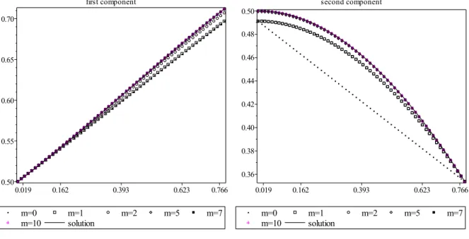
The graphs of the seventh approximation (6.13), (6.14) and of the exact solution (6.9) are shown on Figure6.1.
(a) (b) Figure 6.1: First solution: q=4,m=0, 1, 2, 5, 7, 10.
m ξ1 ξ2 η1 η2
0 0.5000000003 0.4910030682 0.6966729228 0.3535533902 1 0.5000000003 0.4910030705 0.6966729234 0.3535533902 2 0.5000000003 0.4909073352 0.7067944705 0.3535533902 5 0.5000000003 0.4990243859 0.7110836712 0.3535533902 7 0.5000000003 0.4997040346 0.7117894333 0.3535533902 10 0.5000000003 0.4999499916 0.7120202126 0.3535533902 16 0.5000000003 0.4999983385 0.7120583725 0.3535533902 20 0.5000000003 0.4999993608 0.7120592079 0.3535533902 . . . .
∞ 12 12 0.7120595095 0.3535533905
Table 6.1: First solution: values of parameters forq=4.
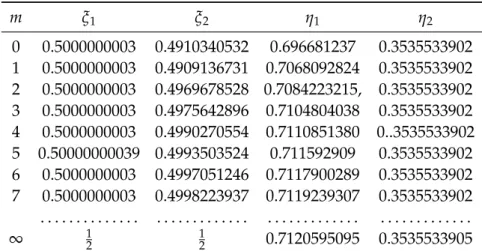
m ξ1 ξ2 η1 η2 0 0.5000000003 0.4910340532 0.696681237 0.3535533902 1 0.5000000003 0.4909136731 0.7068092824 0.3535533902 2 0.5000000003 0.4969678528 0.7084223215, 0.3535533902 3 0.5000000003 0.4975642896 0.7104804038 0.3535533902 4 0.5000000003 0.4990270554 0.7110851380 0..3535533902 5 0.50000000039 0.4993503524 0.711592909 0.3535533902 6 0.5000000003 0.4997051246 0.7117900289 0.3535533902 7 0.5000000003 0.4998223937 0.7119239307 0.3535533902 . . . .
∞ 12 12 0.7120595095 0.3535533905
Table 6.2: First solution: values of parameters forq=11.
m ξ1 ξ2 η1 η2
11 0.4999999999 0.4999103564 0.7120195453 0.3535533905 12 0.4999999999 0.4999501433 0.7120195453 0.3535533905
Table 6.3: First solution: values of parameters forq=17.
Forq=11, the Chebyshev nodes (3.3) on(a,b)have the form
t1 =0.7820385685, t2=0.7555057258, t3=0.70424821007, t4 =0.6317591359, t5 =0.5429785144, t6=0.4439565976, t7=0.3414415658, t8 =0.242419649, t9 =0.1536390274, t10=0.0811499534, t11=0.0298924377, t12 =0.0033595951.
Computing several approximations, we get from (4.15), (4.16) the numerical values for the parameters presented in Table 6.2. Table 6.3 contains the approximate values of parameters forq=17 andm∈ {11, 12}.
6.2 Approximations of the second solution
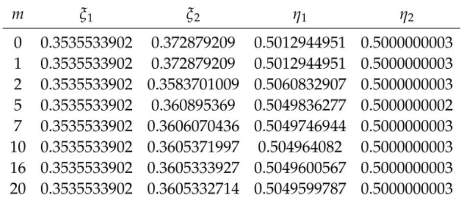
Choosing different constraints when solving the approximate determining system (4.15), (4.16), we find that, along with the root from Table6.1, it has also another root presented in Table6.4.
It is quite evident from the results of computation that this indicates the existence of another solution of the boundary value problem (6.1), (6.2), which is different from (6.9).
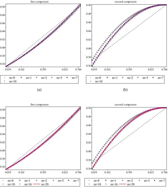
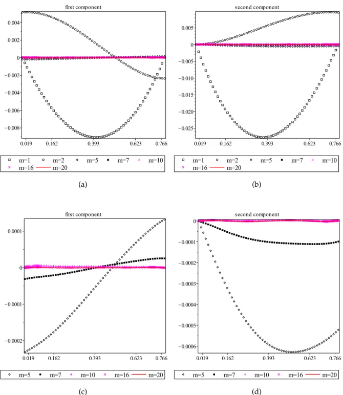
On Figure 6.2, one can see the graph of approximations to the second solution, while Figure6.3 shows the residuals obtained by substituting these approximations into the given differential system (i. e., the functions t 7→ Umk0 (t)− fk(t,Um(t)), k = 1, 2). We see that, e. g., at m = 10, we get a residual of order about 10−5. The computation of 20 approximations withq=4 on a standard portable computer with Intel® Core i3-2310M CPU @ 2.10 GHz takes about 130 seconds.
(a) (b)
(c) (d)
Figure 6.2: Second solution: q=4,m=0, 1, 2, 5, 7, 10, 16, 20.
(a) (b)
(c) (d)
Figure 6.3: The residuals of approximations to the second solution: q = 4, m=1, 2, 5, 7, 10, 16, 20.
m ξ1 ξ2 η1 η2 0 0.3535533902 0.372879209 0.5012944951 0.5000000003 1 0.3535533902 0.372879209 0.5012944951 0.5000000003 2 0.3535533902 0.3583701009 0.5060832907 0.5000000003 5 0.3535533902 0.360895369 0.5049836277 0.5000000002 7 0.3535533902 0.3606070436 0.5049746944 0.5000000003 10 0.3535533902 0.3605371997 0.504964082 0.5000000003 16 0.3535533902 0.3605333927 0.5049600567 0.5000000003 20 0.3535533902 0.3605332714 0.5049599787 0.5000000003
Table 6.4: Second solution: values of parameters forq=4.
Acknowledgements
The work was supported in part by RVO: 67985840 (A. Rontó) and Czech Science Foundation, Project No.: GA16-03796S (N. Shchobak).
References
[1] S. S. Dragomir, The Ostrowski’s integral inequality for Lipschitzian mappings and ap- plications, Comput. Math. Appl. 38(1999), No. 11–12, 33–37. https://doi.org/10.1016/
S0898-1221(99)00282-5;MR1729802
[2] V. L. Goncharov, Theory of interpolation and approximation of functions (in Russian), Moscow: GITTL, 2nd ed., 1954.MR0067947
[3] I. P. Natanson,Constructive function theory. Vol. III. Interpolation and approximation quadra- tures, New York: Frederick Ungar Publishing Co., 1965.MR0196342
[4] A. Ostrowski, Über die Absolutabweichung einer differentiierbaren Funktion von ihrem Integralmittelwert (in German), Comment. Math. Helv. 10(1937), No. 1, 226–227. https:
//doi.org/10.1007/BF01214290;MR1509574
[5] G. M. Phillips,Interpolation and approximation by polynomials, CMS Books in Mathemat- ics/Ouvrages de Mathématiques de la SMC, Vol. 14. Springer-Verlag, New York, 2003.
https://doi.org/10.1007/b97417;MR1975918
[6] T. J. Rivlin,An introduction to the approximation of functions, Blaisdell Publishing Co. Ginn and Co., Waltham, Mass.-Toronto, Ont.-London, 1969.MR0249885
[7] T. J. Rivlin, The Chebyshev polynomials, Wiley-Interscience [John Wiley & Sons], New York–London–Sydney, 1974.MR0450850
[8] M. Rontó, J. Mészáros, Some remarks on the convergence of the numerical-analytical method of successive approximations, Ukrain. Math. J.48(1996), No. 1, 101–107. https:
//doi.org/10.1007/BF02390987;MR1389801
[9] A. Rontó, M. Rontó, Successive approximation techniques in non-linear boundary value problems for ordinary differential equations, in:Handbook of differential equations: ordinary