Weed species composition of small-scale farmlands bears a strong crop-
1
related and environmental signature
2
3
K NAGY *, A LENGYEL †, A KOVÁCS *, D TÜREI ‡, AM CSERGŐ § & G PINKE * 4
5
* Faculty of Agricultural and Food Sciences, Széchenyi István University, 6
Mosonmagyaróvár, Hungary 7
† MTA Centre for Ecological Research, Tihany, Hungary 8
‡ European Molecular Biology Laboratory – European Bioinformatics Institute, Hinxton, UK 9
§ School of Natural Sciences, Trinity College Dublin, Dublin, Ireland 10
11 12 13
Received: 13 February 2017 14
Revised version accepted: 2 October 2017 15
16 17
Running head: Environmental signatures of small-scale farming 18
19 20 21
Correspondence: K Nagy, Széchenyi István University, Faculty of Agricultural and Food 22
Sciences, H-9200 Mosonmagyaróvár, Vár 2, Hungary. Tel: (+36) 70 4019399; Fax: (+36) 96 23
566610; E-mail: galnagykatalin@gmail.com 24
25 26
Word count = 6398 27
Summary 28
29
Weed species loss due to intensive agricultural land use has raised the need to understand 30
how traditional cropland management has sustained a diverse weed flora. We evaluated to 31
what extent cultivation practices and environmental conditions affect the weed species 32
composition of a small-scale farmland mosaic in Central Transylvania (Romania). We 33
recorded the abundance of weed species and 28 environmental, management and site context 34
variables in 299 fields of maize, cereal and stubble. Using redundancy analysis we revealed 35
22 variables with significant net effects, which explained 19.15% of the total variation in 36
species composition. Cropland type had the most pronounced effect on weed composition 37
with a clear distinction between cereal crops, cereal stubble and hoed crops. Beyond these 38
differences, the environmental context of croplands was a major driver of weed composition, 39
with significant effects of geographic position, altitude, soil parameters (soil pH, texture, salt 40
and humus content, CaCO3, P2O5, K2O, Na and Mg) as well as plot location (edge vs core 41
position) and surrounding habitat types (arable field, road margin, meadow, fallow, ditch).
42
Performing a variation partitioning for the cropland types one by one, the environmental 43
variables explained most of the variance compared with crop management. In contrast, when 44
all sites were combined across different cropland types, the crop specific factors were more 45
important in explaining variance in weed community composition.
46 47
Keywords: Transylvania, weed flora, arable fields, agroecology, agro-ecosystem, altitude, 48
field edges, redundancy analysis 49
50
Introduction 51
52
Changes in farming systems, mechanization, increases in field size as well as the use of 53
chemical fertilisers and herbicides have had a marked negative impact on weed species 54
diversity and abundance (Marshall et al., 2003, Albrecht et al., 2016). Many European 55
countries have reported significant decrease in abundance or even extinction of typical arable 56
weed species (Storkey et al., 2011).
57 58
Despite their potential importance for the health of agricultural ecosystems, weed 59
species may also cause significant economical losses for farmers and weed control can be the 60
most expensive agricultural practice aimed at improving crop production (Marshall et al., 61
2003). In order to develop efficient, sustainable and environmentally friendly weed control 62
practices, it is urgent to understand the drivers of weed presence and abundance on cultivated 63
lands (Swanton et al., 1999). We need to investigate how the interaction between farming and 64
weed management systems and the environment affects the composition of weed vegetation 65
in different croplands (Pyšek et al., 2005, Pinke et al., 2011, 2012, 2013).
66 67
Existing evidence is mixed, suggesting that the weed composition of arable lands may 68
primarily be determined by ecological factors (Lososová et al., 2004) or by human activity 69
(Fried et al., 2008, Andreasen & Skovgaard, 2009, Cimalová & Lososová, 2009, Pinke et al., 70
2012). It is however sensible to expect that the two types of factors interact, and the 71
prevalence of one or the other is context-dependent. For instance, where environmental 72
conditions are less favourable to cropping, the degree of agricultural intensification is also 73
lower and the environmental imprint on weed composition is strong (Lososová et al., 2004, 74
Nowak et al., 2015). In upland areas the frequency of herbicide treatments is usually lower 75
than elsewhere (Pál et al., 2013), the proportion of alien weed species is lower and weed 76
species richness is higher (Lososová et al., 2004). Nevertheless, the composition of the weed 77
flora also depends on the crop type, including the division between winter- and summer-sown 78
crops and crop-specific management (Fried et al., 2008). Superimposed on this pattern may 79
be the often-reported increase of weed species richness towards field margins, due to a lower 80
competition pressure from crops and release from chemical stressors in border areas (Seifert 81
et al., 2015). The role of these marginal cropland habitats in conservation is very important 82
and increasingly recognised (Wrzesień & Denisow, 2016). Rare weed species are usually 83
restricted to the outermost few metres of the croplands, where weed species richness and 84
cover are higher compared to the field centre (Wilson & Aebischer, 1995, Fried et al., 2009).
85
The study fields in our area were characteristically small, potentially magnifying this affect as 86
the boundary/area ratio would be increased.
87 88
In many parts of Eastern Europe, the traditional management practices have been 89
preserved for longer compared to Western Europe, conserving important arable biodiversity 90
in small-scale mosaic landscapes (Loos et al., 2015). Although significant land use changes 91
are currently underway (Nyárádi & Bálint, 2013, Loos et al., 2015), due to the high number 92
of small farmlands and a high variety of cropping practices, these landscapes still provide 93
ideal ground for gauging the imprints of environment on weed composition in agricultural 94
lands.
95 96
In this study we investigated the relative effect of agricultural management and 97
environmental factors on weed species composition of arable fields in small-scale farmlands.
98
Our study system was a mosaic of small farmlands in Central Transylvania (Romania) 99
characterised by a high diversity of cropping practices. Detailed surveys of weed vegetation 100
of arable lands in the area have been scarce and the existing studies provided little 101
mechanistic understanding of the persistence of weed species in traditional landscapes 102
(Chirilă, 2001, Ciocârlan et al., 2004, Loos et al., 2015).
103 104
We performed a comprehensive survey of weed vegetation in this area and examined 105
the effects of 14 management-, 12 environment- and two site context variables on species 106
composition of weed communities. We hypothesized that, due to the persistence of traditional 107
management practices and the small-scale farms, the weed composition of arable lands would 108
carry a strong imprint of environmental factors in addition to the effect of management 109
techniques.
110 111 112
Materials and Methods 113
114
Site description 115
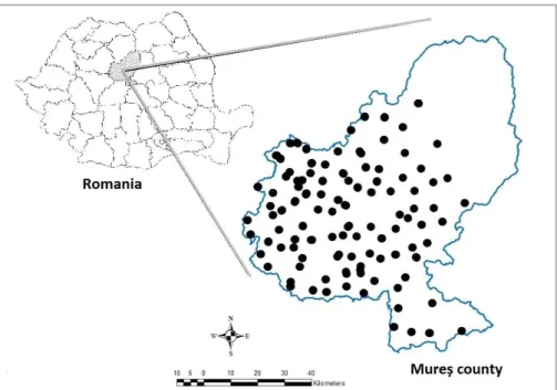
We carried out our survey in 2013 in Central Transylvania, Romania (23°59’260” – 116
26°11’992” North, 46°08’520” – 46°54’597” East), covering nearly the total area of 6714 117
km2 of Mureş county in this region (Fig. 1). The proportion of agricultural land in this county 118
is 61%, of which 54% is classified as arable land. The most widely cultivated crops are 119
cereals and maize (INS, 2016).Our study covered an elevational gradient ranging between 120
260–543 m (Table 1). The lower elevations included the Transylvanian Plateau, more suitable 121
for agriculture due to wide valleys and a milder climate. The higher elevation North-Eastern 122
corner of the county consisted of the Călimani and Gurghiu Mountain foothills, where arable 123
fields were rarer. Here, the temperature and precipitation regimes have been less suitable for 124
crop production and therefore agricultural intensification has been lower, e.g. 4-6 times lower 125
doses of chemical fertilisers and herbicides in average compared to France or Germany 126
(Storkey et al., 2012).
127 128 129
Fig. 1 near here 130
131
Data collection 132
We selected a total of 299 arable fields for the survey in a broadly random pattern, but also 133
depending on farmer’s cooperation (Fig. 1). Within each field we sampled weed vegetation in 134
six randomly selected, 4 m2 plots (2×2 m), totaling 1794 plots. Three plots were located on 135
the field edge (within 2 m from the outermost seed drill line), and three were in the field 136
centre. 101 fields were cereal crops (74 Triticum aestivum L., 11 Triticosecale x rimpaui 137
Wittm., 8 Hordeum vulgare L., 5 Hordeum distichon L., 3 Avena sativa L.) and 97 maize 138
(Zea mays L.). The remaining 101 sites were stubbles of cereal fields. While cereal stubbles 139
are not crops, we analysed them as a separate cropland type due to their unique weed 140
vegetation (Pinke et al., 2010). We surveyed the cereal fields between May 10 and June 6, 141
and the maize and the cereal stubble fields between July 31 and August 20 to ensure that we 142
captured the most comprehensive set of weed species within each cropland type.
143 144
Within each 4 m2 plot, we estimated visually the percentage ground cover of all 145
species, including crop species, and the vegetation data recorded was subsequently digitized 146
and stored in TURBOVEG format (Hennekens & Schaminée, 2001). In addition, we 147
interviewed landowners for information on crop management of each investigated field. We 148
recorded the cropping history (indicating the preceding crop as either cereal or hoed crop), 149
the amount of organic manure applied, whether farmers used chemical fertilisers (N, P2O5, 150
K2O), as well as crop sowing season (previous fall or spring) and field size. Information on 151
weed management (type of herbicides used and number of times mechanical weed control 152
treatments were applied) were also recorded. Herbicides applied on less than 10 fields out of 153
the total of 299 were subsequently dropped from the analyses. To reduce the number of 154
management categories, the ’cropland type’ variable was coded as cereal crop, maize crop or 155
cereal stubble.
156 157
We used soil chemical and physical properties as local environmental variables. From 158
each field we collected one soil sample of 1,000 cm3 from the top 10 cm layer. Soil samples 159
were air dried and stored at room temperature until further analyses were performed at UIS 160
Ungarn GmbH (Mosonmagyaróvár, Hungary). Soil variables included: soil pH, texture, salt 161
and humus content, CaCO3, P2O5, K2O, Na and Mg. In addition, we used three proxies of 162
regional environmental conditions quantified as the geographic latitude, longitude and 163
elevation above sea level of each field, as recorded by a GPS device.
164 165
Finally, we considered two site variables: plot location (edge or field core) and 166
neighbouring habitat (arable field, road margin, meadow, fallow or ditch) to represent 167
composite management and environmental effects.
168 169
Overall we recorded 28 parameters: two site variables, 12 environmental variables 170
and 14 management variables (Table 1).
171 172
Table 1 near here 173
174
Statistical analyses 175
Prior to analyses we averaged the abundance of species across field edge and field core plots 176
respectively, which we subsequently transformed following the Hellinger approach 177
(Legendre & Gallagher, 2001). We also transformed the categorical variables (the amount of 178
chemical fertilisers and herbicides) into ‘dummy’ indicator variables.
179 180
To analyse the relationship between the composition of weed vegetation and site, 181
environmental and management variables, we performed a Redundancy Analysis (RDA).
182
RDA links species abundance data to explanatory variables more accurately than the 183
commonly used Canonical Correspondence Analysis (CCA), even when species responses to 184
environmental gradients are unimodal (Legendre & Gallagher, 2001). Only species with >10 185
occurrences were involved in the analyses. We reduced the number of explanatory variables 186
using stepwise backward selection with a P<0.05 threshold. With this procedure six variables 187
were eliminated: soil pH, Na and salt content, mechanical weeding and herbicides 2,4 D and 188
bromoxinil, resulting in a reduced RDA model with 22 terms with significant effects. The 189
generalised variance inflation factor GVIF (Fox & Monette, 1992) ranged between 1.0 and 190
5.51, indicating no serious collinearity between explanatory variables.
191 192
We then compared the gross and net effects of each explanatory variable, following 193
the methodology described in Lososová et al. (2004). The gross effects represented the 194
variation explained by a ’univariate’ RDA containing the predictor of interest as the only 195
explanatory variable. The net effect was calculated using a partial RDA (pRDA), which 196
included the variable of interest as explanatory variable and the other 21 variables as 197
conditional variables (‘co-variables’). We extracted the explained variance and the adjusted 198
R-squared ( ) for models of both gross and net effects of each variable. In models of net 199
effects, model fit was also assessed by the F-value for which a type I error rate was estimated 200
using 999 permutation tests of the constrained axis. The importance of each explanatory 201
variable was ‘ranked’ using the values of the pRDA (i.e. net effect) models.
202
Subsequently, we identified the 10 species with the highest fit for each explanatory variable.
203 204
We report only the RDA ordination diagrams of the reduced model with the finally 205
selected 22 variables. In these diagrams, continuous variables were represented by their linear 206
constraints, while positions of categorical variables were calculated by weighted averaging of 207
coordinates of plots representing each level.
208 209
In addition, we performed a variation partitioning analysis to assess the relative 210
effects of site, environmental and management variables on weed species composition either 211
within each cropland type separately or across all the fields, and separated by edge vs. centre 212
position (Borcard et al., 2011). This procedure identifies unique and shared contributions of 213
groups of variables using adjusted R-squared values.
214 215
Statistical analyses were performed using the vegan (version 2.3-3) and car (version 216
2.0-25) packages in R 3.1.2 (R Development Core Team). Species fit on the constrained 217
ordination axes was calculated using the ‘inertcomp’ function of vegan package.
218 219
2
Radj
2
Radj
220
Results 221
222
Across the 1794 plots sampled from 299 arable fields we found a total of 141 weed species, 223
110 in cereals, 88 in stubble fields and 76 in maize crops. From the top most threatened 48 224
arable weeds in Europe (Storkey et al., 2012) only four occurred in our dataset, all in cereal 225
fields. Their frequency of occurrence ranged between 1.0 and 9.7% (Adonis aestivalis L.
226
9.7%, Centaurea cyanus L. 6.1%, Ranunculus arvensis L. 5.9%, Lathyrus aphaca L. 1.0%).
227 228
The full RDA model comprising all 28 explanatory variables explained 20.25% of the 229
variance, while the reduced model with 22 explanatory variables still explained 19.15% of 230
the total variation in species composition. All 22 variables (cropland type, geographic 231
position, altitude, soil parameters, plot location and neighbouring habitat) had significant net 232
effects at a P<0.05 level (Table 2). Weed species with the strongest responses to these factors 233
are listed in Tables S1, S2, and S3 in Supporting Information.
234 235
Table 2 near here 236
237
In the reduced RDA ordination (Fig. 2) the first two axes explained 7.65% and 2.51%
238
of the total variation, respectively. Cropland type (cereal crop, maize crop and cereal stubble) 239
resulted in the largest distinction in weed species composition, followed by the sowing season 240
(autumn and spring) (9.46 and 3.84 % of explained variation respectively; Table 2). Species 241
positively associated with the first axis were typical of maize crops (e.g. Amaranthus 242
retroflexus L., Chenopodium album L., Hibiscus trionum L.), while species characteristic of 243
cereal crops were negatively associated with the first axis (e.g. Galium aparine L., Papaver 244
rhoeas L., A. aestivalis). Species found in cereal stubbles had a positive weight on the second 245
axis (e.g. Stachys annua L., Anagallis arvensis L. and Setaria viridis (L.) P. Beauv) (Fig. 2).
246
Neighbouring habitat (a site variable) was the next best important predictor of variation in 247
weed composition (net effect: 0.76% and gross effect: 1.42% explained variation; Table 2).
248
Arable fields were positively, and road margins and meadows were negatively associated 249
with the first axis, while ditches weighted positively on the second axis.
250 251
Further variables with a strong weight on the first axis were organic manure and soil 252
properties (calcium, potassium and humus content), while variables with strong weight on the 253
second axis were soil texture, chemical fertilisers and latitude (Table 2, Fig. 2).
254 255
Fig. 2 near here 256
257
The variation partitioning within each cropland type revealed that environmental 258
variables outperformed the management and site variables, with nearly equal values in 259
stubbles and maize, and slightly lower in cereals (6.6%, 6.5% and 4.8% respectively Fig. 3).
260
The management variables had the highest relative effect in maize and equally lower in 261
cereals and stubbles. The relative effects of site and management variables were similar in 262
cereals (2.5% vs. 2.6% respectively), but in maize and stubbles site explained only a tiny 263
fraction of the variance (0.9–0.2%) (Fig. 3). Variation partitioning over all the 299 fields 264
resulted the highest influence of management variables, being largely driven by crop type, 265
explaining three times more of the total variance compared to the environmental variables 266
(10.9% vs. 3.4%) (Fig. 4). The variation partitioning of the RDA according to the plot 267
location revealed that the effect of environmental variables is only slightly higher in field 268
edges than in the cores (3.2% vs. 2.6% respectively), while the influence of management was 269
nearly equal (10.4% vs. 10.5) (Fig. 5).
270 271
Fig. 3, 4, 5 near here 272
273 274
Discussion 275
Farmland management practices such as cropland type, fertilisation and sowing season were 276
the major drivers of weed composition in the studied system. However, environment and site 277
effects were also important contributors to the revealed patterns. Our report represents the 278
most exhaustive assessment to date of the weed vegetation of arable lands in Central 279
Transylvania, showcasing factors that structure weed composition under agronomical 280
practices currently typical of Eastern Europe.
281 282
Management effect 283
We found that 11 of the 22 significant predictors of weed composition were elements of the 284
management system. From all management variables involved in the study only three (two 285
herbicides and frequency of mechanical weeding) were dropped during the backward 286
selection process, and the effect of all of the remaining management variables were 287
significant. Of these, cropland type had the most pronounced effect, reinforcing the view that 288
crop type is a primary driver of weed vegetation (Cimalová & Lososová, 2009). This can be 289
explained by major differences in cultivation practices between cereals and hoed crops 290
(Andreasen & Skovgaard, 2009, Nowak et al., 2015). Cereal fields are exposed to mechanical 291
disturbance (and stresses caused by herbicides) only at the beginning of the season and after 292
harvesting, ensuring a longer undisturbed growing period for weeds in comparison to hoed 293
crops. Most rare and endangered species (such as A. aestivalis, C. cyanus, L. aphaca, R.
294
arvensis in our dataset) have been associated with cereals, because they germinate mainly in 295
autumn and have their life cycle adapted to that of cereals rather than to that of hoed spring 296
sown crops (Kolářová et al., 2013). Following cereal harvest, stubbles are left undisturbed 297
until late autumn, leaving open sunny habitats suitable for the establishment of species that 298
are able to germinate at high temperatures and tolerate summer drought, e.g. summer 299
therophytes (S. annua, A. arvensis, Kickxia elatine (L.) Dumort.). In contrast, species 300
identified as typical of maize crops have their germination associated with later crop sowing 301
date (Gunton et al., 2011) and able to tolerate continuous disturbance regimes (Echinochloa 302
crus-galli (L.) P. Beauv, Setaria pumila (Poir.) Schult., H. trionum, C. album) (Fig. 2). A 303
typical disturbance-tolerance strategy is the steady germination ability of seeds throughout 304
the cultivation period (Fried et al., 2012).
305 306
It would have been interesting to distinguish between the effect of the season (using 307
the date of observation) and the effect of the management. However, these two factors are 308
confounded in the one variable, cropland type, making impossible their separate analysis. It is 309
likely that season and management interacted to shape the characteristics we associated with 310
stubble in our analysis. Despite similar sowing dates of cereals, subsequent germination later 311
in the season would have contributed to the different floras recorded in their stubble.
312
Preceding management regimes, i.e. cropping technologies applied in cereals and maize, also 313
have their impact on weed floras. Furthermore, environmental conditions in the stubble are 314
different, e.g. free from the shading. Accordingly, not only the flora of cereals and that of 315
their stubbles differs remarkably, but stubble and maize also have different weed flora, even 316
though the fact that they were surveyed in the same season. Consequently, stubble is not a 317
homogenous category among cropland types; its subdivision and introduction of season as a 318
new variable would have made possible to further dissect the causalities behind the patterns 319
of weed composition.
320 321
Fertilisation was an important filter of weed species and a selective driver of weed 322
abundance (for similar results see Lososová et al., 2006, Pinke et al., 2012, Seifert et al., 323
2015). Several species responded to organic manure with increased abundances (e.g.
324
Convolvulus arvensis L., S. pumila, E. crus-galli), while chemical fertilisers could be linked 325
to higher abundances of only three species (Rubus caesius L., H. trionum, Elymus repens (L.) 326
Gould). Almost all weed species that responded positively to higher organic manure were 327
associated with maize fields (e.g. E. crus-galli, C. album, A. retroflexus), due to higher doses 328
applied in hoed crops (Lososová et al., 2006).
329 330
A strong negative relationship between field size and weed diversity at the landscape 331
level has often been reported due to a higher associated heterogeneity of cultivated areas and 332
a larger edge / area ratio in smaller field sizes (Marshall et al., 2003, Gaba et al., 2010, Fahrig 333
et al., 2015). Some mechanical operations are less efficient in smaller fields and farmers 334
cultivating small fields tend to have limited access to weed management technology or 335
expertise (Pinke et al., 2013). In our study this effect, albeit significant, was less pronounced 336
(field size ranked only 12th among the explanatory variables), as our data covers only a 337
narrow range of field sizes (most fields in our survey were small, 59% had ≤1 ha).
338 339
The sowing season was an important driver of weed composition in our survey, where 340
we investigated winter- and spring-sown cereals and spring sown maize. Winter annual weed 341
species (Veronica persica Poir., Consolida orientalis (J. Gay) Schrödinger, G. aparine, P.
342
rhoeas) were strongly associated with autumn-sown cereals, while summer annual weed 343
species (A. retroflexus, C. album, H. trionum, S. pumila, E. crus-galli) preferred spring-sown 344
cultures, many of the latter being typical weeds of hoed crops (Fig. 2). These results concur 345
with earlier evidence, confirming that the presence of multiple crops and cropping times may 346
considerably increase the regional weed species pool (Marshall et al., 2003, Pinke et al., 347
2011, Fried et al., 2012, Vidotto et al., 2016).
348 349
Among preceding crops, winter cereals usually favour winter annuals, while hoed 350
crops summer annuals. In our analysis preceding crop ranked only the 15th among the 351
predictors, not independently from the common practice in the surveyed area to alternate 352
winter cereals with hoed crops. The rotation of cereals and hoed crops aims to interrupt the 353
build-up of weed populations associated with particular crop types (de Mol et al., 2015).
354 355
We found that the use of herbicides significantly affects the occurrence and 356
abundance of weed species. The active ingredients of the herbicides with significant effect 357
were fluoroxypyr, florasulam, isoxaflutol with ciprosulfamid, thiencarbazone-methyl and 358
dicamba (Table 2). All of these were used for post-emergence control. Florasulam, 359
fluoroxypyr and dicamba can be used against dicotyledonous weeds, and isoxaflutol + 360
ciprosulfamid and thiencarbazone-methyl are broad-spectrum herbicides for the control of 361
both monocotyledons and dicotyledonous weeds. Although we identified several weed 362
species that were correlated with herbicides according to their explained variation in the 363
constrained axes, without a survey before and after herbicide treatment we cannot draw firm 364
conclusions on the effect of herbicides. Accordingly, these correlations are not shown in the 365
supporting information.
366 367
Environmental effect 368
We found nine environmental variables with significant net effects on weed composition, 369
including both regional and local factors (Table 2).
370 371
Longitude ranked the 2nd, altitude the 3rd and latitude the 13th among all predictors.
372
These variables have been used as proxies of regional climate conditions such as precipitation 373
and mean temperature (Lososová et al., 2004, 2006, Hanzlik & Gerowitt, 2011, de Mol et al., 374
2015). Species strongly associated with lower altitudes were troublesome weeds such as 375
Solanum nigrum L., Xanthium italicum Moretti, Polygonum aviculare L. and R. caesius, 376
while species correlated with higher altitudes were cereal weeds typical of traditional 377
farming, e.g. C. orientalis, C. cyanus. This pattern has often been reported from agricultural 378
landscapes situated in heterogeneous geographic conditions (Lososová et al., 2004, Pál et al., 379
2013, Nowak et al., 2015). The north-eastern higher altitude part of our study area is less 380
favourable especially for maize but also for other crops, as a consequence the cultivation is 381
less intense (Fig. 1). We interpret the change in weed composition along this geographical 382
gradient as a result of both environmental effects and differences in farming methods 383
between lowland and upland areas due to environmental constraints.
384 385
As expected, soil physical and chemical properties such as texture, Ca, K, Mg, P and 386
humus content exerted significant effects on the occurrence of certain weed species (Pinke et 387
al., 2012, 2016). For example we found that Cirsium arvense (L.) Scop., a species common in 388
all crop types, preferred soils with high humus and Mg content, but avoided alkaline soils.
389
Although in many studies pH was a crucial determinant of weed species presence (e.g. Pyšek 390
et al., 2005, Fried et al., 2008, Vidotto et al., 2016), other investigations, including ours, 391
found this factor to be non-significant (see also Nowak et al., 2015), likely because neutral 392
soils were dominantly prevalent in our study area.
393 394
Site effect 395
The plot location (edge vs core position) and the neighbouring habitat type had moderate 396
effects on weed composition (the 6th and the 14th most important predictors, respectively).
397
Most weeds preferred field edges and only one species, C. arvensis had higher abundance 398
towards field interiors. It is well known from other agricultural ecosystems that crop margins 399
support higher species richness and the principle is applied in weed conservation (e.g. Pinke 400
et al., 2012, Kolářová et al., 2013, Seifert et al., 2015, Wrzesień & Denisow, 2016).
401
Mechanisms behind these patterns include the crop’s lower competition ability, dilution or 402
lack of chemical stressors in the border areas (Seifert et al., 2015), release from competition 403
for light exerted by crop species (Pinke et al., 2012) and a higher external propagule supply 404
from adjacent habitats (Gaba et al., 2010, Conceptión et al., 2012, Pinke et al., 2012, 405
Wrzesień & Denisow, 2016).
406 407
In our mosaic of small farmlands, neighbouring habitats were diverse (arable field, 408
ditch, fallow, meadow, road margin) and were linked to the presence/abundance of specific 409
weeds in the crop fields. Maintaining a diversity of non-farmed habitats adjacent to farmlands 410
may therefore result in an enriched weed flora in crop fields. Here we have shown that this 411
externally driven enrichment diminishes substantially towards field interiors (see also Gaba et 412
al., 2010, Pinke et al., 2012).
413 414 415
Environment vs management factors 416
In the variation partitioning within each cropland type the environmental variables explained 417
the largest fractions of the variance, which is in accordance with the results of previous 418
studies (Lososová et al., 2004, Pinke et al., 2012, 2016, de Mol et al., 2015). The effect of 419
environmental variables reached the highest proportion in cereal stubbles, explaining two and 420
a half time more variance than the effect of management variables. This may be due to the 421
lack of particular cropping practices on stubbles. In maize crops the relative influence of 422
environmental variables was similarly high. Both maize and stubble represented the late 423
summer weed flora, and the higher contributions of environment could be due to the longer 424
period following weed management practices, which allows the weed vegetation to recover 425
from the seed banks primarily under the influence of soil and climatic conditions.
426
Furthermore, in maize the management variables explained a higher proportion of variance in 427
weed communities when compared to cereals and stubbles possibly due to the frequently 428
repeated cultivation tasks typical of maize crops.
429 430
In contrast to the crop specific analyses the variation partitioning carried out over all 431
sites highlighted the importance of the management variables. This shows that the 432
involvement of crop type can increase the contribution of management remarkably, 433
highlighting the generally powerful impact of crop-related factors on the weed flora (Fried et 434
al., 2008, Gunton et al., 2011).
435 436
Splitting up the variance allocated to the plot location, the management factors 437
account for approximately three times more variance compared to the environmental 438
variables both in field cores and edges. We found no difference between field edges and cores 439
in the importance of management variables, contrary to the findings of Pinke et al. (2012).
440
This could be explained by the generally small field sizes in this study, where the cultural and 441
ecological conditions between edge and core are likely to be more similar than in the large 442
fields (Wilson & Aebischer, 1995).
443 444
Acknowledgements 445
The publication is supported by the EFOP-3.6.3-VEKOP-16-2017-00008 project. The project 446
is co-financed by the European Union and the European Social Fund.
447 448
References 449
450
ALBRECHT H,CAMBECÈDES J,LANG M & WAGNER M (2016) Management options for rare 451
arable plants in Europe. Botany Letters 164, 389-415.
452
ANDREASEN C & SKOVGAARD IM (2009) Crop and soil factors of importance for the 453
distribution of plant species on arable fields in Denmark. Agriculture, Ecosystems and 454
Environment 133, 61-67.
455
BORCARD D, GILLET F & LEGENDRE P (2011) Numerical Ecology with R. Springer, New 456
York Dordrecht London Heidelberg.
457
CHIRILĂ C(2001)Biologia buruienilor. Ceres, Bucureşti, România.
458
CIMALOVÁ Š & LOSOSOVÁ Z (2009) Arable weed vegetation of the northeastern part of the 459
Czech Republic: effects of environmental factors on species composition. Plant 460
Ecology 203, 45–57.
461
CIOCÂRLAN V,BERCA M,CHIRILĂ C,COSTE I& POPESCU G(2004)Flora segetală a 462
României. Ceres, Bucureşti, România.
463
CONCEPTIÓN ED,FERNÁNDEZ-GONZÁLEZ F&DÍAZ M(2012)Plant diversity partitioning in 464
Mediterranean croplands: effects of farming intensity, field edge, and landscape 465
context. Ecological Applications 22, 972-981.
466
FAHRIG L,GIRARD J,DURO D,PASHER Jet al. (2015) Farmlands with smaller crop fields have 467
higher within-field biodiversity. Agriculture, Ecosystems and Environment 200, 219- 468
234.
469
FOX J& MONETTE G(1992) Generalized collinearity diagnostics. Journal of the American 470
Statistical Association 87, 178-183.
471
FRIED G,KAZAKOU E& GABA S(2012) Trajectories of weed communities explained by traits 472
associated with species response to management practices. Agriculture, Ecosystems and 473
Environment 158, 147-155.
474
FRIED G, NORTON LR & REBOUD X (2008) Environmental and management factors 475
determining weed species composition and diversity in France. Agriculture, Ecosystems 476
and Environment 128, 68–76.
477
FRIED G,PETIT S,DESSAINT F& REBOUD X(2009)Arable weed decline in Northern France:
478
Crop edges as refugia for weed conservation? Biological Conservation 142, 238-243.
479
GABA S,CHAUVEL B,DESSAINT F,BRETAGNOLLE V&PETIT S(2010)Weed species richness 480
in winter wheat increases with landscape heterogeneity. Agriculture, Ecosystems and 481
Environment 138, 318-323.
482
GUNTON RM,PETIT S& GABA S(2011)Functional traits relating arable weed communities to 483
crop characteristics. Journal of Vegetation Science 22, 541-550.
484
HANZLIK K & GEROWITT B (2011) The importance of climate, site and management on weed 485
vegetation in oilseed rape in Germany. Agriculture, Ecosystems and Environment 141, 486
323–331.
487
HENNEKENS SM& SCHAMINÉE JH(2001)TURBOVEG, a comprehensive database 488
management system for vegetation data. Journal of Vegetation Science 12, 587-591.
489
INS(INSTITUTUL NAŢIONAL DE STATISTICĂ –NATIONAL INSTITUTE OF STATISTICS):Available 490
at: http://www.mures.insse.ro/main.php?lang=fr&pageid=420 (last accessed:
491
09.03.2016).
492
KOLÁŘOVÁ M,TYŠER L& SOUKUP J(2013) Impact of site conditions and farming practices 493
on the occurrence of rare and endangered weeds on arable land in the Czech Republic.
494
Weed Research 53, 489-498.
495
LEGENDRE P & GALLAGHER ED (2001) Ecologically meaningful transformations for 496
ordination of species data. Oecologia 129, 271–280.
497
LOOS J,TURTUREANU PD, VON WEHRDEN Het al. (2015) Plant diversity in a changing 498
agricultural landscape mosaic in Southern Transylvania (Romania). Agriculture, 499
Ecosystems and Environment 199, 350-357.
500
LOSOSOVÁ Z,CHYTRÝ M,CIMALOVÁ Šet al. (2004) Weed vegetation of arable land in 501
Central Europe: Gradients of diversity and species composition. Journal of Vegetation 502
Science 15, 415–422.
503
LOSOSOVÁ Z,CHYTRÝ M,KÜHN Iet al. (2006) Patterns of plant traits in annual vegetation of 504
man-made habitats in central Europe. Perspectives in Plant Ecology, Evolution and 505
Systematics 8, 69-81.
506
MARSHALL EJP,BROWN VK,BOATMAN ND,LUTMAN PJW,SQUIRE GR&WARD LK(2003) 507
The role of weeds in supporting biological diversity within crop fields. Weed Research 508
43, 77-89.
509
DE MOL F, VON REDWITZ C & GEROWITT B (2015) Weed species composition of maize fields 510
in Germany is influenced by site and crop sequence. Weed Research 55, 574–585.
511
NOWAK A, NOWAK S, NOBIS M & NOBIS A (2015) Crop type and altitude are the main 512
drivers of species composition of arable weed vegetation in Tajikistan. Weed Research 513
55, 525–536.
514
NYÁRÁDI I&BÁLINT J(2013) Erdély gyomnövényzete, gyomproblémák, védekezési 515
lehetőségek. Gyomnövények, gyomirtás 14, 25-34.
516
PÁL RW,PINKE G,BOTTA-DUKÁT Zet al. (2013) Can management intensity be more 517
important than environmental factors? A case study along an extreme elevation gradient 518
from central Italian cereal fields. Plant Biosystems 147, 343-353.
519
PINKE G,BLAZSEK K,MAGYAR Let al. (2016) Weed species composition of conventional 520
soyabean crops in Hungary is determined by environmental, cultural, weed 521
management and site variables. Weed Research 56, 470-481.
522
PINKE G, KARÁCSONY P, BOTTA-DUKÁT Z & CZÚCZ B (2013) Relating Ambrosia 523
artemisiifolia and other weeds to the management of Hungarian sunflower crops.
524
Journal of Pest Science 86, 621–631.
525
PINKE G, KARÁCSONY P, CZÚCZ B, BOTTA-DUKÁT Z & LENGYEL A (2012) The influence of 526
environment, management and site context on species composition of summer arable 527
weed vegetation in Hungary. Applied Vegetation Science 15, 136–144.
528
PINKE G,PÁL R& BOTTA-DUKÁT Z(2010)Effects of environmental factors on weed species 529
composition of cereal and stubble fields in western Hungary. Central European Journal 530
of Biology 5, 283-292.
531
PINKE G, PÁL RW, TÓTH K, KARÁCSONY P, CZÚCZ B & BOTTA-DUKÁT Z (2011) Weed 532
vegetation of poppy (Papaver somniferum) fields in Hungary: effects of management 533
and environmental factors on species composition. Weed Research 51, 621–630.
534
PYŠEK P,JAROŠÍK V,KROPÁČ Z,CHYTRÝ M,WILD J& TICHÝ L(2005) Effects of abiotic 535
factors on species richness and cover in Central European weed communities.
536
Agriculture, Ecosystems and Environment 109, 1-8.
537
SEIFERT C,LEUSCHNER C& CULMSEE H(2015) Arable plant diversity on conventional 538
croplands – The role of crop species, management and environment. Agriculture, 539
Ecosystems and Environment 213, 151-163.
540
STORKEY J,MEYER S,STILL KS& LEUSCHNER C (2012) The impact of agricultural 541
intensification and land-use change on the European arable flora. Proceedings of the 542
Royal Society B: Biological Sciences 279, 1421-1429.
543
SWANTON CJ,SHRESTHA A,ROY RC,BALL-COELHO BR& KNEZEVIC SZ(1999) Effect of 544
tillage systems, N, and cover crop on the composition of weed flora. Weed Science 47, 545
454-461.
546
VIDOTTO F, FOGLIATTO S, MILAN M & FERRERO A (2016) Weed communities in Italian 547
maize fields as affected by pedo-climatic traits and sowing time. European Journal of 548
Agronomy 74, 38–46.
549
WILSON P& AEBISCHER N(1995)The distribution of dicotyledonous arable weeds in relation 550
to distance from the field edge. Journal of Applied Ecology 32, 295-310.
551
WRZESIEŃ M& DENISOW B(2016) The effect of agricultural landscape type on field margin 552
flora in south eastern Poland. Acta Botanica Croatica 75, 217-225.
553
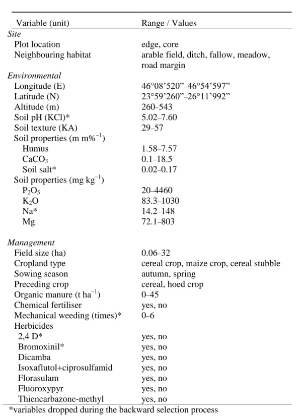
Table 1 Units and ranges of continuous variables and values of categorical variables recorded 554
on each cropland for this study.
555 556
Variable (unit) Range / Values
Site
Plot location edge, core
Neighbouring habitat arable field, ditch, fallow, meadow, road margin
Environmental
Longitude (E) 46°08’520”–46°54’597”
Latitude (N) 23°59’260”–26°11’992”
Altitude (m) 260–543
Soil pH (KCl)* 5.02–7.60
Soil texture (KA) 29–57 Soil properties (m m%–1)
Humus 1.58–7.57
CaCO3 0.1–18.5
Soil salt* 0.02–0.17
Soil properties (mg kg–1)
P2O5 20–4460
K2O 83.3–1030
Na* 14.2–148
Mg 72.1–803
Management
Field size (ha) 0.06–32
Cropland type cereal crop, maize crop, cereal stubble
Sowing season autumn, spring
Preceding crop cereal, hoed crop Organic manure (t ha–1) 0–45
Chemical fertiliser yes, no Mechanical weeding (times)* 0–6 Herbicides
2,4 D* yes, no
Bromoxinil* yes, no
Dicamba yes, no
Isoxaflutol+ciprosulfamid yes, no
Florasulam yes, no
Fluoroxypyr yes, no
Thiencarbazone-methyl yes, no
*variables dropped during the backward selection process 557
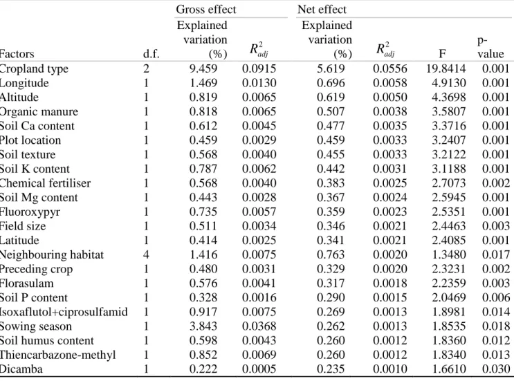
Table 2 Gross and net effects of the explanatory variables on the weed species composition 558
identified using (p)RDA analyses with single explanatory variables 559
560
Factors d.f.
Gross effect Net effect Explained
variation (%)
2
Radj
Explained variation (%)
2
Radj F p-value
Cropland type 2 9.459 0.0915 5.619 0.0556 19.8414 0.001
Longitude 1 1.469 0.0130 0.696 0.0058 4.9130 0.001
Altitude 1 0.819 0.0065 0.619 0.0050 4.3698 0.001
Organic manure 1 0.818 0.0065 0.507 0.0038 3.5807 0.001
Soil Ca content 1 0.612 0.0045 0.477 0.0035 3.3716 0.001
Plot location 1 0.459 0.0029 0.459 0.0033 3.2407 0.001
Soil texture 1 0.568 0.0040 0.455 0.0033 3.2122 0.001
Soil K content 1 0.787 0.0062 0.442 0.0031 3.1188 0.001
Chemical fertiliser 1 0.568 0.0040 0.383 0.0025 2.7073 0.002
Soil Mg content 1 0.443 0.0028 0.367 0.0024 2.5945 0.001
Fluoroxypyr 1 0.735 0.0057 0.359 0.0023 2.5351 0.001
Field size 1 0.511 0.0034 0.346 0.0021 2.4463 0.003
Latitude 1 0.414 0.0025 0.341 0.0021 2.4085 0.001
Neighbouring habitat 4 1.416 0.0075 0.763 0.0020 1.3480 0.017
Preceding crop 1 0.480 0.0031 0.329 0.0020 2.3231 0.002
Florasulam 1 0.576 0.0041 0.317 0.0018 2.2359 0.003
Soil P content 1 0.328 0.0016 0.290 0.0015 2.0469 0.006
Isoxaflutol+ciprosulfamid 1 0.917 0.0075 0.269 0.0013 1.8981 0.014
Sowing season 1 3.843 0.0368 0.262 0.0013 1.8535 0.018
Soil humus content 1 0.598 0.0043 0.260 0.0012 1.8360 0.012 Thiencarbazone-methyl 1 0.852 0.0069 0.260 0.0012 1.8340 0.013
Dicamba 1 0.222 0.0005 0.235 0.0010 1.6610 0.030
561
562
Fig. 1 The distribution of the surveyed arable fields across the study area (Mureș county, 563
Central Transylvania, Romania). At this scale individual points may represent a number of 564
fields with different cropland types.
565 566
567
568
569
570
Fig. 2 Ordination diagrams of the reduced RDA model containing the 22 significant 571
explanatory variables and the species. Only the species with the highest weight on the 572
first two RDA axes are presented.
573 574
575
Fig. 3 Percentage contributions of groups of explanatory variables to the variation in weed 576
species composition in the three investigated cropland types, identified by variation 577
partitioning (only non-negative adjusted R-squared values are shown).
578
579
Fig.4 Percentage contributions of groups of explanatory variables to the variation in weed 580
species composition using all the 299 fields, identified by variation partitioning (only non- 581
negative adjusted R-squared values are shown).
582 583 584
585
Fig. 5 Percentage contributions of groups of explanatory variables to the variation in weed 586
species composition in field edges and field cores, identified by variation partitioning 587
(only non-negative adjusted R-squared values are shown).
588 589
Supporting Information 590
591
Additional Supporting Information may be found in the online version of this article:
592
Table S1 Names, fit and score values of species giving the highest fit along the first 593
constrained axis in the partial-RDA models of the significant environmental variables 594
specified in Table 2. (Only the most abundant ten weed species are shown).
595
Table S2 Names, fit and score values of species giving the highest fit along the first 596
constrained axis in the partial-RDA models of the significant management variables specified 597
in Table 2. (Only the most abundant ten weed species are shown).
598
Table S3 Names, fit and score values of species giving the highest fit along the first 599
constrained axis in the partial-RDA models of the significant site variables specified in Table 600
2. (Only the most abundant ten weed species are shown).
601