Joint analysis of active and passive surface wave methods – case studies from seismic microzonation of Budapest
Erzsébet Győri1, Máté Timkó2, Zoltán Gráczer3, Gyöngyvér Szanyi4
Kövesligethy Radó Seismological Observatory, Geodetic and Geophysical Institute, Research Centre for Astronomy and Earth Sciences, Budapest, Hungary,
gyori@seismology.hu1, timko@seismology.hu2, graczer@seismology.hu3, szanyi@seismology.hu4
ABSTRACT: Local soil conditions can significantly amplify damages caused by earthquakes. Knowledge of shear wave velocities is essential when this amplification is computed or soil classes are determined during application of earthquake safety standards. The present study shows some examples of seismic site characterization that were performed during seismic microzonation of Budapest. To determine shear wave velocities, we have carried out both active (MASW) and passive (ESAC, ReMi) surface wave measurements in different parts of the city. In order to reveal the possible subsoil resonance H/V ratios were computed based on microseismic noise measurements. Our other purpose was to study the local applicability of ambient noise cross-correlation method in noisy urban environment. To increase the reliability of the results, joint inversion of different types of dataset and/or full velocity spectra inversion were performed. Performance of the applied methods depended on the local circumstances.
Keywords: shear-wave velocity; surface wave methods; horizontal-to-vertical spectral ratio; ambient noise cross- correlation; joint inversion
1. Introduction
Seismicity around Budapest is moderate but somewhat higher than the average in Hungary. The largest well known historical earthquake (M5.6) occurred in 1956, in the vicinity of Dunaharaszti, 5-10 km distance from the southern boundary of the capital. The quake caused damages in Budapest that were surveyed in detail after the event. Studying damage distribution, some areas of more severe than the average damages could be observed (Fig. 1). The average in a given point was computed using the average intensity attenuation computed only for this event. Direct use of these data requires great precautions but obviously contain the effect of local geology. For example, bad condition of houses caused larger damages while lack of damages can indicate not only less damages but unbuilt areas in that time too. Therefore, we thoroughly have examined the correlation of these areas with the geological structures, local subsoil conditions, groundwater levels, built-up of the area and with the quality of buildings located there.
The geological structure of Budapest is very complex which potentially has a great impact on damage distribution. On the right bank of the Danube (Buda side), older Triassic and Miocene rocks form the Buda Hills while Holocene and Pleistocene sediments cover the area on the left bank (Pest side). Generally, it can be stated that although some dots with higher intensity can be seen in Buda, but characteristically the Buda side was less damaged during the quake. The areas with more serious damages are mainly located in the Pest side but their distribution is not even.
In the frame of this project, we have studied the applicability of different seismic surface wave methods that could be used for microzonation purposes within the area of a large city. The test sites were selected on the basis of geological conditions and damage distribution of the 1956 Dunaharaszti earthquake.
We have carried out active (Multichannel Analysis of Surface Waves – MASW) and passive (Refraction Microtremor – ReMi, Extended Spatial AutoCorrelation – ESAC) seismic measurements to determine the S wave velocities of upper sedimentary layers. Where the field conditions allowed, we have applied all of the aforementioned methods. In every test site microseismic noise measurements were also carried out and joint inversion of surface wave dispersion and horizontal-to- vertical spectral ratio (HVSR) curves were performed.
We have studied also the local applicability of ambient noise correlation method (seismic interferometry), because the resulted velocity model can supplement the model determined by MASW and ESAC measurements in larger depths.
Figure 1. Differences of reported and “expected” intensities caused by the Dunaharaszti earthquake on the map of Budapest. The
studied sites are delineated by squares.
2. Applied methods
2.1. Active and passive seismic measurements
All MASW, ReMi and ESAC methods are shallow seismic techniques, which allow to determine the shear wave velocity by measuring the propagation of the surface waves at several sensors on the free surface. The main contribution to the surface waves is given by the Rayleigh waves that are dispersive in stratified media.
Dispersion means that the phase or group velocities depend on the frequency. This circumstance implies that high frequency waves with relatively short wavelengths contain information about the upper part of the site, while low frequency waves with longer wavelengths provide information about the deeper layers. Active methods often lack clear information in the low frequency range.
Passive techniques supplement them in identifying the velocities in larger depths because microseismic background noise can contain more low frequency component.
In the MASW method [1] that is an active seismic technique, the surface waves were generated by an 8 kg hammer. The wave motion was measured along a linear array of 24 pcs 4.5 Hz vertical geophones. The geophone distances were 3 and 4 m; the minimum offsets at the MASW measurements were 15 m and 20 m respectively.
The recorded traces from multiple shocks were stacked to attenuate incoherent noise. The ReMi measurements [2] were performed using the same linear geophone array as was used by the MASW. Because locations of sources are necessarily unknown during passive measurements, the consequence is that the obtained velocity spectra must be interpreted as “lower velocity bound”. In order to eliminate the directivity effects during ReMi measurements, L-shaped arrays were used for the ESAC [3] measurements.
Data processing consisted of the following steps: 1) determination of the velocity spectrum from the measured seismic traces. Velocity spectrum is a matrix that represents the propagation velocity as a function of frequency. It is mathematically derived from seismic traces so it is an objective entity without any sort of interpretation from the user. 2) Interpretation of velocity spectrum in the form of modal or effective dispersion curves of Rayleigh waves. The effective dispersion curve is the apparent dispersion curve resulting from the dispersion of all the modes and is represented by the peaks or the lower velocity border (in case of ReMi approach) on the velocity spectrum. 3) Calculation of the numerical apparent dispersion curve from an initial model. 4) Inverting the apparent dispersion curve in order to find the best fitting model so the vertical shear wave profile of the site.
Interpretation of velocity spectrum in the form of modal dispersion curves raises different problems.
Different subsurface velocity models can have very similar modal dispersion curves. The fundamental mode is not necessarily the dominating one and the continuity of a signal in the velocity spectrum does not necessarily mean that it pertains to a single mode. Therefore,
misinterpretation of the data in terms of modal dispersion curves is extremely high.
To overcome the above mentioned problems, two types of approximation were followed.
Surface wave measurements were supplemented by microseismic noise measurements and HVSR curves [4]
were computed in every locations. The method is sensitive to shear wave velocity contrasts but completely different velocity models can produce nearly identical HVSR curves. It can be used to estimate average shear wave velocities only if depths of these contrasts are known. Since HVSR and surface wave dispersion are two different aspects of the same phenomena, i.e. the surface wave propagation, there is difference in their nonuniqueness. Therefore we jointly inverted the phase dispersion and HVSR curves to reduce the risk of misinterpretation. We applied a MOEA (Multi-Objective Evolutionary Algorithms) procedure driven by the Pareto optimality [5]. Basically this is performed by keeping separate the two considered misfits and by determining the "goodness" of a model by computing its position according to the Pareto dominance criterion [6].
The second approach was the application of full velocity spectrum (FVS) inversion procedure that considers the velocity spectrum as a whole and can be somehow regarded as a sort of extended effective dispersion curve approach. It allows the full exploitation of all the modes present in the field data (and without their interpretation in terms of modal dispersion curves) thus resulting in a very-well constrained inversion procedure capable of providing a robust subsurface VS
model.
2.2. Ambient noise correlation method
Ambient noise correlation method [7] was also tested because of its numerous advantages. It can be carried out without an active source and using only two seismometers, which can be placed even on streets in urban areas. It uses the cross-correlation of two, simultaneously recorded seismograms to infer the impulse response of the medium between the two receivers. The cross-correlation function is used to generate dispersion curves, which can be inverted for S wave velocities. The application of the noise correlation method has been spreading rapidly because of its numerous advantages. Besides studying the structure and velocities of Earth’s crust and mantle [8, 9], microseismic noise tomography can also be applied for S wave velocity determination of shallow surface layers [10].
In the frame of this project, we have examined the applicability of the method in local scale and carried out noise measurements at all sites where the seismic measurements were performed. The interstation distance between the simultaneously recording instruments varied from 40 m to 1.2 km. The measurement time was between 30 minutes and 2 hours depending on the interstation distance (the shorter measurement times belonged to the shorter distances). In a typical measurement setting we used three seismometers at the same time. This arrangement provided three station pairs for which we could determine the cross-correlation functions (CCFs).
The cross-correlation functions were used to obtain the dispersion curves and estimate surface wave group velocities. In order to retrieve the dispersion curves, the processing procedure of ambient noise data consists of four main steps [11]: 1) preprocessing, 2) cross- correlation and stacking, 3) measurement of dispersion curves and 4) quality control.
Different methods were tested for the processing steps of correlation analysis and stacking and the best combination of them was selected to retrieve the cross- correlation functions and the dispersion curves. Data preparation begun with removing the mean and trend followed by frequency filtering. For time-domain normalization the one-bit normalization technique was applied.
The second phase is the cross-correlation computation and stacking of correlation functions. We have tested the conventional correlation method and the phase cross- correlation (PCC) method [12] as well. PCC improves the SNR of the cross-correlation function. It is more sensitive to waveform similarity and less sensitive to large amplitude phenomena than the conventional cross- correlation and it does not require time-domain normalization. Therefore, we omitted the normalization step when PCC was applied. Two types of stacking techniques have been tested: the standard linear stacking, which is used in most of the ambient noise tomography studies and time-frequency phase weighted stacking described by [13], which has been applied in some recent ambient seismic noise tomography studies. Various combinations of the previously described processing steps have been used to calculate the cross-correlation functions. We've compared the SNR ratio of the obtained cross-correlation functions and concluded that phase correlation with phase weighted stacking leads to the highest SNR.
We have determined group velocity dispersion curves for the CCFs computed from vertical, radial and transversal component of noise recordings. The group velocity dispersion curves determined from vertical and radial component recordings belong to Rayleigh waves, while the ones obtained from transversal noise components correspond to the Love waves. The group velocity dispersion curves were obtained using the frequency-time analysis (FTAN) method.
The resulted velocity model can supplement the model determined by MASW and ESAC measurements in larger depths.
2.3. Determination of resonances by microseismic noise based HVSR technique
VS30 values used to determine soil classes in earthquake safety standards doesn’t explain entirely the damage distribution caused by earthquakes. These don’t give information about the resonance of the subsoil, the possible topographic and 2-3D focusing effects.
Resonance can be expected in case of large impedance contrast i.e. where large velocity hard rock is covered by loose sediments. Resonance frequency depends on the thickness and average shear wave velocity in the upper
loose layers while the strength of the resonance depends on the impedance contrast. A special soil class “E” in Eurocode 8 earthquake safety standard marks this type of subsoils.
We have performed microseismic noise measurements on the area to identify and delineate the areas where resonance can occur. We have determined the resonance frequencies and the strength of the resonance by computing horizontal-to-vertical spectral ratio (HVSR) curves [4].
Because of the size of the studied area, we have to restrict the measurements to those areas where large impedance contrasts are expected on the basis of geological maps or where damages during Dunaharaszti earthquake were larger than the average. So we have carried out microseismic noise measurements in 275 points within the boundaries of the city using three Le3D/5s type mobile seismographs and Güralp datalogger.
In addition, every active and passive Vs measurements were supplemented by microseismic noise measurements to reveal the possible subsoil resonance and to improve the reliability of the resulted shear wave velocity profile by joint inversion of the two types of dataset.
Processing of active and passive seismic data, computation of H/V ratios have been done by WinMASW software [14].
3. Results
This paper presents the performed measurements and results obtained at three locations. In two cases the measurement sites were selected on the basis of above- average damages experienced during the Dunaharaszti earthquake, in one case due to unfavorable soil conditions.
3.1. Városliget
Damages caused by the 1956 Dunaharaszti earthquake were larger than the average at the southeast corner of the Városliget (Fig. 1). According to the available geological maps and borehole data, low bearing capacity peat can be found in shallow depth on the area (Fig. 2.) so our purpose was to determine the shear wave velocity of these strata. Because of the available free park area, we could perform MASW, ReMi and ESAC measurements.
These were supplemented with microseismic noise measurements to calculate HVSR curves and apply the cross-correlation method.
Dispersion curve of Rayleigh-waves was determined primarily from velocity spectrum of MASW measurement. The source was a hammer so the low frequency part of the spectrum is quite uncertain.
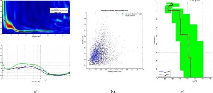
Therefore low frequency part of the apparent dispersion curve was picked with the help of velocity spectra of the two passive methods (Fig. 3). After that we have performed the joint inversion of H/V and dispersion curves (Fig. 4) using genetic algorithm. Fig. 4b shows the bi-objective space with a cloud of misfits of the models showing that the inversion process is highly consistent (Pareto front analysis).
However it has to be note that while the velocity spectrum is objective and mathematically obtained from the seismic traces without any personal interpretation, dispersion curves are the results of a subjective interpretation. The velocity spectrum shows the superposition of fundamental and higher modes therefore an erroneous picking of modal dispersion curves necessarily leads to meaningful results. Therefore we have also performed Full Velocity Spectra (FVS) inversion in every measurement location. The results of the FVS inversion performed on a MASW measurement can be seen in Fig. 5. The resulted VS profile is very similar to the profile of Fig. 4c; a low velocity layer (less than 150 m/s) can be seen above 5 m which probably indicate the existence of a low strength peat layer. Above the peat there is a liquefiable sandy layer, where the VS
also does not exceed 200 m/s. Nonetheless the values of VS30 were 285 and 290 m/s in the two cases so the soil category is “C” according to the classification of Eurocode 8. It is an average soil class which does not show the unfavorable properties of the upper layers and the larger damages experienced during the Dunaharaszti earthquake.
Noise cross-correlation measurements were performed on the same area as the active and passive seismic measurements. We calculated cross-correlation functions between 9 pairs of stations with different interstation distances. Examining the results, the ratio of good quality CCFs was around 85 % for transversal component and 40 % for the vertical and radial
components. Fig. 6a shows the CCF that was computed from vertical components of two seismometers which were in 309 m distance from each other. Group velocity dispersion curve of Rayleigh-wave (Fig. 6b) was determined from this cross correlation function. On the left side of Fig. 6c, the red lines show the best fitting velocity-depth functions while on the right side their misfit values with the picked group velocity curve can be seen. Although the resolution of the depth-velocity function determined using noise cross correlation method is lower than the resolution given by seismic methods, it could give information about the velocities of larger depths.
Figure 2. Geological profile [15] at the location of surface wave measurements carried out in Városliget
Figure 3. ReMi and ESAC velocity spectra with the apparent dispersion curves
a) b) c)
Figure 4. a) Rayleigh wave velocity spectrum computed from MASW measurement (up) and the H/V curve (down). The picked dispersion curve was determined using the velocity spectrum of all three types of measurements (MASW, REMI, ESAC). b) bi-objective space with a cloud of misfits
of the models c) the resulted VS profile with the search space FILL
SAND
PEAT SILT
CLAY
Measurements
REMI ESAC
Figure 5. Results of full velocity spectrum inversion in Városliget.
a)
c)
b)
Figure 6. Determination of velocity profile using ambient noise cross correlation method in Városliget: a) cross-correlation function, b) group velocity curve of Rayleigh wave and c) the results of inversion
3.2. Lágymányos and Ördögárok
The investigation of the Lágymányos area (southern part of Fig. 7) that is located directly next to the Danube, was justified by the fact that a lake was found in the area in the 1880s. In the 20th century, it was filled up, mainly with the debris of Second World War. Presently there are university and office buildings in the area, but in 1956 at the time of the Dunaharaszti earthquake, it was largely unbuilt.
In the area, Kiscell Clay of the early Oligocene age is found at a depth of about 20 to 30 m. This impermeable
layer had been the bottom of the Lágymányos Lake.
Above it, Holocene alluvium of the Danube, clayey gravel and sandy soils can be found, which vary in thickness and it is gradually thinning to the west. Just below the surface, 7–9 m thick anthropogenic fill is located. For this reason, we considered this area unfavorable from earthquake engineering point of view.
To determine shear wave velocity profile, MASW, ReMi, ESAC measurements were also performed in the area. In addition to shallow seismic measurements, microseismic background noise measurements were
carried out at several points. We calculated the noise cross-correlation and HVSR curves too.
Throughout the area, two peaks appeared on the HVSR curves, which indicates two larger velocity contrasts. The one could be seen between 0.8 and 1.2 Hz and the other was between 3.5 and 4.5 Hz. One example is shown in Fig. 7. The joint inversion of the dispersion and HVSR curves resulted VS velocities of 160–190 m/s in artificial fill, 250–300 m/s in fluvial deposits and 400–
500 m/s in the Oligocene Kiscell Clay. The formation of the higher frequency peak was due to the velocity increase at the boundary of the Holocene fluvial sediments and the Oligocene clay. The lower frequency peak around 1 Hz can be due to a deeper velocity contrast, but this could not be identified due to the lower penetration of our measurements and the lack of deeper boreholes. Depth of the Mesozoic bedrock in the area is 400-500 m, so the expected resonance should have appeared at a frequency of less than 1 Hz.
Figure 7. An example of HVSR curves computed from the microseismic noise measurements performed in Lágymányos
area
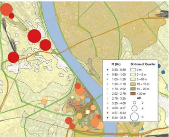
Fig. 8 shows the higher resonant frequencies determined from the measurements performed in Lágymányos (southern part). Diameter of the points is proportional with the amplitude of resonance peak while their color shows their frequency. The higher frequency resonance peaks are plotted together with the thickness map of the Quaternary formations. The figure clearly shows the correlation between the quaternary thickness and the resonance frequencies.
Noise cross-correlation measurements were performed also in the area. Cross-correlation functions between 9 pairs of stations with different interstation distances were calculated. Lágymányos region located near the river Danube and the measurements were carried out between large buildings and in the presence of significant traffic. In this case we have not found good quality CCFs in the case of vertical and radial components and the ratio of the good quality transversal component CCFs was only around 10 %.
The VS30 values were between 300 and 320 m/s so the soil class was “C” according to Eurocode 8 in the area but the low velocity in the artificial fill indicates its compressibility that necessitates deeper foundation.
Micro-seismic noise measurements were also carried out in the area of Ördögárok (northwestern part in Fig.
8). The area is the valley of Ördögárok-stream that
separates the Castle Hill from the Gellért Hill and Nap Hill. In this area, Triassic dolomite is covered by thin alluvial deposits of the Ördögárok-strem. The low sediment thickness and strong impedance contrast are well illustrated by the high, 6-8 Hz resonance frequency of and its high peak amplitude (around 8-10). Our measurements have shown that significant amplification can be expected in the valley, in the high frequency range during earthquakes.
Figure 8. Locations of measuring points in Lágymányos (southern part) and Ördögárok (northwestern part) plotted on the quaternary thickness map of the studied area. Diameter of the
circles is proportional with the amplitude of resonance peak while their color shows their frequency.
3.3. Hűvösvölgy
Hűvösvölgy is one of the areas where damages during Dunaharaszti earthquake were larger than in the neighboring areas and the residents report stronger than the average shaking also during recent earthquakes. The area is located in a tectonic valley which is filled with Holocene sediments of variable thickness.
We carried out microseismic noise measurements in the area to study the resonance properties of the valley.
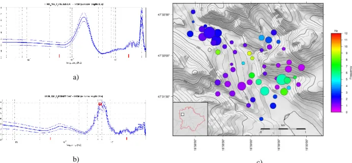
We computed the average HVSR curves (Fig. 9) and determined the azimuthal variations of horizontal-to vertical ratios (Fig. 10) which is useful for the recognition of site response directivity.
We have found strong resonance in some locations that can explain the larger damage at the time of the earthquake. However, the resonance frequencies of the soil are coincident with the resonance frequencies of the current buildings only in the SE part of the area. Probably this soil-building interaction appears in the relatively large number of felt reports that have arrived into the Observatory during recent earthquakes.
Drawing the polarity diagrams onto a topographic map, amplification of topography moreover the effect of the valley edge could be also detected (Fig. 10).
a)
b) c)
Figure 9. Examples of H/V curves (a, b) and measurement points plotted on the topographic map of the studied area (d). The colors show the resonance frequencies while the size of the circles is proportional with the amplitude of resonance peaks. The high frequency peaks in the valley
show the 1D resonance of the quaternary stream sediments while the low frequency ones arise from deeper structures or from lateral amplifications.
a)
c) b)
Figure 10. a) Multiple resonance peaks on H/V curve and b) the directivity plot indicate the directional amplification. The computations were made for location indicated by the small arrow. (The maximum frequency on the directivity plots is 20 Hz. The frequency axis on the polar plot is linear.) c) Directivity diagrams plotted on the topographic
map of the studied area
4. Summary and conclusions
The present study showed some examples of seismic site characterization that were performed during seismic microzonation of Budapest. To determine shear wave velocities, we performed both active (MASW) and passive (ESAC, ReMi) surface wave measurements in different parts of the city. We studied the local applicability of ambient noise cross-correlation method in noisy urban environment performing simultaneous microseismic noise measurements using seismometers that were placed at different distances.
In order to reveal the possible subsoil resonance HVSR curves were computed on the basis of microseismic noise measurements. Our other purpose was to study the local applicability of ambient noise cross-correlation method in noisy urban environment.
Usually the MASW and ESAC measurements provided good results, velocity spectra computed form them were clear and well usable. In case of ReMi measurements, distribution of noise sources strongly influenced the appearance of velocity spectra. The color scale of the spectrum may also influence the designation of apparent dispersion curve so its interpretation was much more subjective.
The measurements were processed first separately but because sometimes the result of inversion are not unequivocal, we have performed joint inversion of different types of measured data.
Reliability of velocities increased by joint inversion of different type of dataset. But we could not find one exclusively preferable methodology that would be the best in every circumstances. In case of mode jumps often the Full Velocity Spectra (FVS) inversion gave the most realistic results but in other cases picking of dispersion curve gave better results. One of our experiences was that the value of VS30 was quite stable even if the different processing methods resulted different VS profiles.
Our other experiences were that even if the engineering geological maps indicated unfavorable subsoil conditions at the measurement points, the soil category was always “C” on the basis of VS30 value (this can be regarded as an “average” soil type in Hungary).
We have studied the local applicability of ambient noise cross correlation method and have concluded that the quality of the results depends strongly on the location of the measurements. We have got miscellaneous results;
the quality of CCFs was better in more quiet environments, far from strong seismic noise sources.
If we consider all of the measurements (regardless of the location within the territory of Budapest), 60 % of the transversal CCFs can be considered of good quality. In the case of vertical and radial CCFs this ratio is much lower, it is around 30 %. Making a distinction between the densely and sparsely built/populated areas we can find a significant difference between ratios of good quality CCFs. This phenomenon unfortunately limits the applicability of the method in urban environments.
We carried out microseismic noise measurements in Budapest and identified areas prone to soil resonance.
These areas can be found mainly in the valleys and hill- side areas in Buda side. In case of some locations soil- building resonance were also manifested.
Acknowledgement
The project presented in this article is supported by the Hungarian Scientific Research Fund under Grant OTKA K105399 and K81295. Tibor Czifra from the Kövesligethy Radó Seismological Observatory and students from Department of Geophysics and Space Science of ELTE were actively taken part in the measurements.
References
[1] Park, C. B., Miller, R. D., & Xia, J. “Multichannel analysis of surface waves”, Geophysics, 64(3), pp. 800-808, 1999.
https://doi.org/10.1190/1.1444590
[2] Louie, J.N. “Faster, better: Shear-wave velocity to 100 meters depth from Refraction Microtremor arrays”, Bulletin of the Seismological Society of America, 91, pp. 347–364.
2001.https://doi.org/10.1785/0120000098
[3] Asten, M.W. “Geological control on the three-component spectra of Rayleigh-wave microseisms”, Bulletin of the Seismological Society of America, 68, pp. 1623–1636, 1978.
[4] Nakamura, Y. “A method for dynamic characteristics estimation of subsurface using microtremor on the ground surface”, Railway Technical Research Institute, Quarterly Reports, 30(1), 1989.
[5] Li, H., Zhang, Q. “Multiobjective optimization problems with complicated Pareto sets, MOEA/D and NSGA-II”, IEEE
transactions on evolutionary computation, 13(2), pp. 284-302.
2008. https://doi.org/10.1109/TEVC.2008.925798
[6] Dal Moro, G. “Insights on surface wave dispersion and HVSR:
joint analysis via Pareto optimality”, Journal of Applied
Geophysics, (72)2, pp. 129-140, 2010.
https://doi.org/10.1016/j.jappgeo.2010.08.004
[7] Shapiro, N. M., Campillo, M. “Emergence of broadband Rayleigh waves from correlations of the ambient seismic noise”, Geophysical Research Letters, 31(7). 2004.
https://doi.org/10.1029/2004GL019491
[8] Szanyi, G., Gráczer, Z., Győri, E. “Ambient seismic noise Rayleigh wave tomography for the Pannonian basin”, Acta Geodaetica et Geophysica, 48, pp. 209–220, 2013.
doi:10.1007/s40328-013-0019-3
[9] Brenguier, F., Shapiro, N. M., Campillo, M., Nercessian, A., Ferrazzini, V. “3‐D surface wave tomography of the Piton de la Fournaise volcano using seismic noise correlations”, Geophysical
Research Letters, 34(2), 2007.
https://doi.org/10.1029/2006GL028586
[10] Picozzi, M., Parolai, S., Bindi, D., Strollo, A. “Characterization of shallow geology by high-frequency seismic noise tomography”, Geophysical Journal International, 176(1), pp. 164-174. 2009.
https://doi.org/10.1111/j.1365-246X.2008.03966.x
[11] Bensen, G. D., Ritzwoller, M. H., Barmin, M. P., Levshin, A. L., Lin, F., Moschetti, M. P., Yang, Y. “Processing seismic ambient noise data to obtain reliable broad-band surface wave dispersion measurements”, Geophysical Journal International, 169(3), pp.
1239-1260, 2007. https://doi.org/10.1111/j.1365- 246X.2007.03374.x
[12] Schimmel, M. “Phase cross-correlations: Design, comparisons, and applications”, Bulletin of the Seismological Society of America, 89(5), pp. 1366–1378, 1999.
[13] Schimmel, M., Gallart, J. “Frequency-dependent phase coherence for noise suppression in seismic array data”, Journal of Geophysical Research: Solid Earth, 112(B04303), 2007.
https://doi.org/10.1029/2006JB004680
[14] Dal Moro, 2014 WinMasw Dal Moro, G. (2014). Surface wave analysis for near surface applications. Elsevier.
[15] VIBROCOMP. “Városliget építési szabályzatról szóló 32/2014.
(VII.) Főv. Kgy. rendelet módosítása, Stratégiai környezeti vizsgálat”, “Amendments of Városliget Building Regulations No.
32/2014(VII.) by Metropolitan Assembly, Strategic Environmental Assessment”, (in Hungarian), [online] Available at: https://docplayer.hu/18254975-Varosliget-epitesi- szabalyzatrol-szolo-32-2014-vii-fov-kgy-rendelet-modositasa- strategiai-kornyezeti-vizsgalat.html [Accessed: 06 12 2019]