Cyclic quadrangles from squares
Zvonko Čerin
a, Gian Mario Gianella
baDepartment of Mathematics, University of Zagreb e-mail: cerin@math.hr
bDipartimento di Matematica, Universita di Torino e-mail: gianella@dm.unito.it
Submitted 6 April 2006; Accepted 7 April 2006
Abstract
In this paper we show how to use computers to discover appearence of cyclic quadrangles in geometric configurations based on a fixed squareABCD and a variable pointP in the plane. The idea is to consider various central points (like the orthocenters) of the four trianglesABP, BCP, CDP and DAP or their orthogonal projections to the lines AP, BP, CP and DP. This is done in Maple V by describing basic functions for the analytic plane geometry and applying them to these configurations. The figures are realized in The Geometer’s Sketchpad, Mathematica, and Maple V.
Keywords: square, triangle, orthocenter, circumcenter, area, Steiner point, cyclic quadrangle
MSC:51N20, 51M04, 14A25,14Q05
1. Introduction
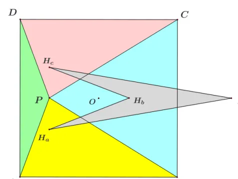
Consider in the plane a positively oriented (in the counterclockwise sense) square ABCD with the center O and a point P which is not on any of the four linesAB,BC,CDandDA. LetHa,Hb,Hc andHd be the orthocenters (i.e., the intersections of altitudes) of the triangles ABP, BCP, CDP and DAP, respec- tively. Let Ja,Jb,Jc andJd denote the orthogonal projections ofHa,Hb,Hc and Hd onto the linesAP,BP,CP andDP, respectively. (See Figures 1 and 2.)
In this paper we want to show how one can use computers to explore properties of the quadranglesHaHbHcHdandJaJbJcJd. The first property of the quadrangle HaHbHcHdthat its diagonalsHaHcandHbHdare perpendicular is obvious because pointsHaandHc are on the perpendicular throughP onto linesABandCDwhile Hb andHd are on the perpendicular throughP onto linesBC andDA.
23
A B D C
O
Ha
Hb Hc
Hd
P
Figure 1: The quadrangleHaHbHcHd from orthocenters.
The second property is more difficult to establish. We shall do this later using analytic geometry. Ever since Decartes this is the most simple and the most effec- tive method to transfer geometric problems into algebraic setting. The reduction usually leads to equations whose solutions give answers. Since the software for symbolic computation (like Derive, Maple V and Mathematica) excels in solving equations, in this way we get the possibility to use computers in our explorations.
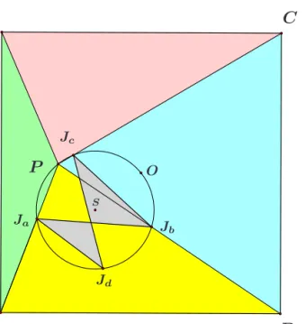
Property 2. The pointsO,P,Ja,Jb,Jc andJd lie on a circle. In particular, the quadrangle JaJbJcJd is cyclic.
We can say more about the circlemwhich appears in the Property 2. It is the circumcircle of the negatively oriented square P ON M built on the segment P O.
Hence, if |P O|=δ, then the radius of the circlemis δ√22 (see Figure 2).
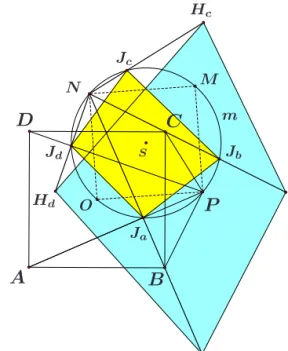
The third property describes the following surprising connection of the quad- ranglesHaHbHcHd andJaJbJcJd(see Figure 3).
Property 3. The linesHaJa,HbJb,HcJc and HdJd intersect in the pointN and go through the points B,C,D andA, respectively.
Now one can wonder when is the quadrangleHaHbHcHd cyclic and when will the quadrangleJaJbJcJdhave perpendicular diagonalsJaJcandJbJd. The answers give the following two theorems.
A B D C
O
Ja
Jb Jc
Jd
S
P
Figure 2: The cyclic quadrangleJaJbJcJd.
Theorem 1.1. The quadrangle HaHbHcHd is cyclic if and only if the point P is either on the line AC, on the line BD or on the circumcircle k of the square ABCD.
Theorem 1.2. In the quadrangle JaJbJcJd the linesJaJc andJbJd are perpendic- ular if and only if the pointP is either on the line AC, on the lineBD or on the circumcirclek of the square ABCD.
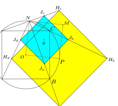
More precisely, Ha =Hc and/or Hb=Hd if and only if P is either on the line AC or on the lineBD. Hence, the first two parts of the locus from Theorems 1.1 and 1.2 correspond to the case when the quadrangle HaHbHcHd degenerates to a segment or a point and either Ja=Jc or Jb=Jd. The role of the third part (the circumcirclek) is explained better by the following statement: IfP is on the circumcirclek, then
(a)HaHbHcHd is a square of side equal to the diagonals ofABCD with P as the center whose diagonalsHaHc andHbHd are parallel to the linesBC andAB, (b)JaJbJcJdis also a square of side equal to the half of the diagonals ofABCD, (c) JaJbJcJd and HaHbHcHd are related by the homothety h(N,2) where N is the vertex of the square on the segmentP O (see Figure 4).
A B D C
O
Ha
Hb Hc
Hd
Ja
Jb Jc
Jd S
P
N M
m
Figure 3: The linesHaJa,HbJb,HcJc andHdJd concur in the pointN.
An interesting path is to explore how the areas of the quadranglesHaHbHcHd
and JaJbJcJd compare to the area Ω of the square ABCD. We define the area
|W XY Z| of the quadrangle W XY Z as the sum |W XY|+|W Y Z| of (oriented) areas of the trianglesW XY andW Y Z.
For every real numberm letPm and Qm denote the loci of all points P such that |HaHbHcHd|=mΩand|JaJbJcJd|=mΩ, respectively.
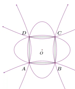
Theorem 1.3. For m <0, m= 0, 0< m <2, m= 2 and m >2 the set Pm is the union of two hyperbolas, the union of lines AC and BD, the empty set, the circumcirclek of the squareABCD, and the union of two ellipsis, respectively. If the axes of one conic areϕandψ then the axes of the other areψ andϕ.
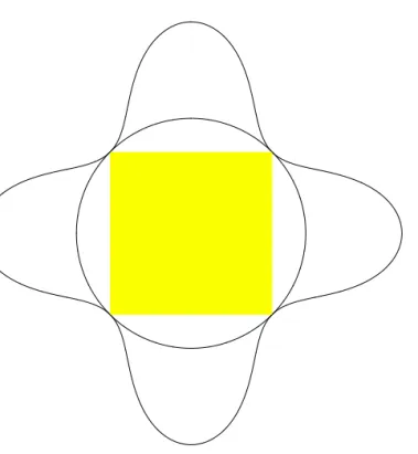
The Figures 5 and 6 show the setsPmfor m=−1 andm= 3 and the setQ1
together with the square ABCD. Notice thatQ1 2
2 is the union of the circumcircle k of the square ABCD and a symmetric curve of order six that touchesk in the vertices of the square.
Let us conclude this description of our results with some comments on what else one can do with this approach. Instead of orthocenters we can consider other central points of the triangle (like the centroid, the circumcenter, the center of the nine-point circle – see the references [3] and [4] for the list of more than thou-
A B D C
O
S
Ha
Hb Hc
Hd
Ja
Jb Jc
Jd
P
M N
Figure 4: The squares HaHbHcHd andJaJbJcJd when the point P is on the cir- cumcircle of ABCD.
sand such points). For example, we have the following analogue of Property 2 for circumcenters.
LetOa,Ob,OcandOdbe the circumcenters of the trianglesABP,BCP,CDP andDAP, respectively. LetNa,Nb,Nc andNddenote the orthogonal projections ofOa,Ob, Oc andOdonto the lines AP,BP,CP andDP, respectively.
Property 4. The pointsNa, Nb,Nc andNd are vertices of the square which is related to the squareABCD by the homothetyh(P, 12).
A computer search reveals that the Steiner point gives the following result also similar to the Property 2.
Recall that the Steiner point is denoted as X(99) in [3] and on page 120 of [1] it is noted that the Steiner point of a triangle is the center of mass of the system obtained by suspending at each vertex a mass equal to the magnitude of the exterior angle at that vertex. It is also the intersection of the circumcircle with the Steiner ellipse and the point of concurrency of parallels through the vertices to the corresponding sides of its first Brocard triangle (see [2]).
LetSa,Sb,Sc andSdbe the Steiner points of the triangles ABP,BCP,CDP andDAP, respectively.
Property 5. The points P,Sa,Sb, Sc andSd lie on a circle whose center is
A B C D
O
Figure 5: The lociP−1 (hyperbolas) andP3(ellipses).
on the lineP O. In particular, the quadrangleSaSbScSd is cyclic.
In this article we took the squareABCD as the underlying figure. Of course, it is possible to take instead any quadrangle or any triangle and perform similar constructions. The possibilities are numerous here but it remains to explore which of these choices give interesting results.
2. Primer on analytic plane geometry in Maple V
The key idea of the analytic geometry is to associate algebraic entities with geometric objects and then investigate them using algebraic methods.
The input of points on the plane in Maple V is quite simple because they are just ordered pairs of real numbers (their rectangular coordinates). For example, the input
tA:=[2, 3]: tB:=[5, 7]: tC:=[-2, 0]: tT:=[x, y]:
defines four points on the plane A(2,3),B(5,7),C(−2,0),T(x, y).
We shall now list definitions of basic functions in Maple V for analytic geometry in the plane in rectangular coordinates. The first group of these functions areFS
Figure 6: The locusQ1 2.
(shortcut for composition of commandssimplifyandfactor),dis(the distance of two points),mid(the midpoint of two points),rat(the point which divides two given points in given ratiok6=−1),rat2(the point which divides two given points in given ratio mn wherem+n6= 0).
FS:=a->factor(simplify(a)):
dis:=(a,b)->FS(sqrt((a[1]-b[1])ˆ2+(a[2]-b[2])ˆ2)):
mid:=(a,b)->FS([(a[1]+b[1])/2,(a[2]+b[2])/2]):
rat:=(a,b,k)->FS([(a[1]+k*b[1])/(1+k),
(a[2]+k*b[2])/(1+k)]):
rat2:=(a,b,m,n)->FS([(n*a[1]+m*b[1])/(m+n),
(n*a[2]+m*b[2])/(m+n)]):
The lines in the program Maple V are represented as ordered triples[a, b, c]of coefficients of their linear equations. For example, the input
pX:=[1, 0, 0]: pY:=[0, 1, 0]: pD:=[1, -1, 0]: pG:=[-1, 2, 2]:
define the y-axis, thex-axis, the bisector of the first and the third quadrant and the line−x+ 2y+ 2 = 0.
We continue with functionsli1(for a line through a given point with a given slope),li2(for a line through two given different points),olQ(to test if a point is
on a line),clQ(to test if three given points are collinear), andins(the intersection of two lines or the information that they are parallel).
li1:=(a,k)->FS([k,-1,a[2]-k*a[1]]):
li2:=(a,b)->FS([a[2]-b[2],b[1]-a[1],a[1]*b[2]-b[1]*a[2]]):
olQ:=(t,p)->FS(t[1]*p[1]+t[2]*p[2]+p[3]):
clQ:=(a,b,c)->FS(a[1]*b[2]-a[1]*c[2]-b[1]*a[2]+
b[1]*c[2]+c[1]*a[2]-c[1]*b[2]):
ins:=(p,q)->FS([(q[3]*p[2]-q[2]*p[3])/(q[2]*p[1]-q[1]*p[2]), (q[1]*p[3]-q[3]*p[1])/(q[2]*p[1]-q[1]*p[2])]):
Functions par andperfor the parallel and the perpendicular through a point to a line and testspaQandpeQif two lines are parallel or perpendicular and the test ccQfor concurrency of three lines (i.e., whether they are parallel or intersect in a point) are next.
par:=(t,p)->FS([p[1],p[2],-t[1]*p[1]-t[2]*p[2]]):
per:=(t,p)->FS([p[2],-p[1],t[2]*p[1]-t[1]*p[2]]):
paQ:=(p,q)->FS(q[1]*p[2]-p[1]*q[2]):
peQ:=(p,q)->FS(p[1]*q[1]+p[2]*q[2]):
ccQ:=(a,b,c)->FS(a[1]*b[2]*c[3]-a[1]*b[3]*c[2]-b[1]*a[2]*
c[3]+b[1]*a[3]*c[2]+c[1]*a[2]*b[3]-c[1]*a[3]*b[2]):
We conclude with the functionsproandarfor the orthogonal projection of a point onto a line and for the oriented area of a triangle on three given points.
pro:=(a,p)->FS([
(p[2]*(a[1]*p[2]-a[2]*p[1])+p[1]*p[3])/(p[1]ˆ2+p[2]ˆ2), (p[1]*(a[2]*p[1]-a[1]*p[2])-p[2]*p[3])/(p[1]ˆ2+p[2]ˆ2)]):
ar:=(a,b,c)->FS((a[2]*c[1]-b[1]*a[2]-a[1]*c[2]+
a[1]*b[2]+b[1]*c[2]-c[1]*b[2])/2):
3. Central points functions
In this continuation of the previous section we shall describe functions for the central points that are mentioned in the introduction: the circumcenter, the ortho- center, and the Steiner point. On the way to define the Steiner point we also need functions for the symmedian point and the vertices of the first Brocard triangle.
First define the functions for the perpendicular bisector of a segment and the triangle circumcenter and orthocenter.
bis:=(a,b)->per(mid(a,b),li2(a,b)):
O_:=(a,b,c)->ins(bis(a,b),bis(a,c)):
H_:=(a,b,c)->ins(per(a,li2(b,c)),per(b,li2(c,a))):
that symmedians bisect sides of the triangle from the projections Ah, Bh, Ch of vertices on opposite sidelines.
Ah_:=(a,b,c)->pro(a,li2(b,c)):
K_:=(a,b,c)->ins(li2(a,mid(Ah_(b,c,a),Ah_(c,a,b))), li2(b,mid(Ah_(c,a,b),Ah_(a,b,c)))):
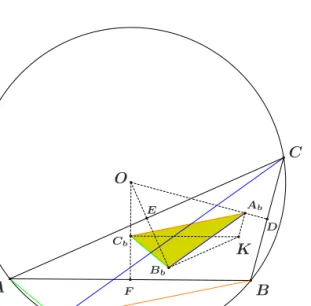
The verticesAb, Bb, Cb of the first Brocard triangle are the orthogonal projections of the symmedian point onto the perpendicular bisectors of sides (see [1, p. 110]
and Figure 7).
Ab_:=(a,b,c)->pro(K_(a,b,c),bis(b,c)):
Hence, the Steiner point is defined as follows (see Figure 8):
S_:=(a,b,c)->ins(par(a,li2(Ab_(b,c,a),Ab_(c,a,b))), par(b,li2(Ab_(c,a,b),Ab_(a,b,c)))):
A B
C
D E
F
O
K
S
Ab
Bb
Cb
Figure 7: The Steiner point S is the intersection of parallels through vertices to sides of the first Brocard triangleAbBbCb.
4. Verification of results
We shall now show how to prove most of the claims from the introduction with the help of computers in Maple V.
We first define the points A, B, C, D, O and P. They will be denoted with small letters becauseDis reserved in Maple V.
a:=[-1,-1]:b:=[1,-1]:c:=[1,1]:d:=[-1,1]:o:=[0,0]:p:=[x,y]:
Then we give the pointsUtforU=H, J, O, N, S andt=a, b, c, d(all points mentioned in the introduction).
Ha:=H_(a,b,p):Hb:=H_(b,c,p):Hc:=H_(c,d,p):Hd:=H_(d,a,p):
Ja:=pro(Ha,li2(a,p)):Jb:=pro(Hb,li2(b,p)):
Jc:=pro(Hc,li2(c,p)):Jd:=pro(Hd,li2(d,p)):
Oa:=O_(a,b,p):Ob:=O_(b,c,p):Oc:=O_(c,d,p):Od:=O_(d,a,p):
Na:=pro(Oa,li2(a,p)):Nb:=pro(Ob,li2(b,p)):
Nc:=pro(Oc,li2(c,p)):Nd:=pro(Od,li2(d,p)):
Sa:=S_(a,b,p):Sb:=S_(b,c,p):Sc:=S_(c,d,p):Sd:=S_(d,a,p):
The proof of the Property 2 is accomplished with the following input.
s:=O_(o,p,Ja):FS(dis(s,o)-dis(s,Jb));
FS(dis(s,o)-dis(s,Jc));FS(dis(s,o)-dis(s,Jc));
Since the output is three times number0(zero), we conclude that the pointsO,P, Ja,Jb,Jc andJd are on a circle. Its centerS gives for the input
peQ(li2(o,s),li2(p,s));
the output 0, so that S is the center of the negatively oriented square P ON M.
Notice that the pointsN andM aren:=rat(p,s,-2): andm:=rat(o,s,-2):.
The proof of the Property 3 requires to see that we get zero as the output of each of the following eight commands.
clQ(n,Ha,Ja); clQ(n,Hb,Jb); clQ(n,Hc,Jc); clQ(n,Hd,Jd);
clQ(b,Ha,Ja); clQ(c,Hb,Jb); clQ(d,Hc,Jc); clQ(a,Hd,Jd);
Proof of Theorem 1.1. The quadrangle HaHbHcHd is cyclic if and only if the distance between the circumcenters of the trianglesHaHbHc andHaHbHdis equal to zero.
dis(O_(Ha,Hb,Hc), O_(Ha,Hb,Hd))ˆ2;
This square of distance is equal to
T(x−y)2(x+y)2 x2+y2−22
x2+y2+ 22
4 (x2−2x+y2)2(y−1)2(y+ 1)2(x−1)2(x+ 1)2(x2+ 2y+y2)2, whereT is the polynomial
x6+ 3x4y2+ 3x2y4+y6−2x5+ 6x4y−8x3y2+ 8x2y3−6xy4+ 2y5+ 2x4
−16x3y+ 12x2y2−16xy3+ 2y4−4x3+ 12x2y−12xy2+ 4y3+ 4x2+ 4y2.
and x2+y2−2 = 0 are equations of the linesAC andBD and of the circumcir- cle k of the square ABCD, the claim of Theorem 1.1 follows provided we prove that the polynomial T is equal to zero only for P from the subset of the union W =AC∪BD∪k.
Let x=rcosθ and y=rsinθ for r>0 and 06θ <2π. Let u and v de- note3(sinθ−cosθ) + sin 3θ+ cos 3θand3−8 sin 2θ−cos 4θ. ThenT =r2U with U =r4+u r3+v r2+ 2u r+ 4. Hence, it remains to show that the real roots of the equation(*) U = 0give points from the setW.
Note thatu2−4v+ 16 = 4(1 + sin 2θ)(4−(sin 2θ−1)2)is always positive ex- cept for θ= 3π4 , 7π4 when it is equal to zero. Letwdenote√
u2−4v+ 16.
Applying the basic commandsolveto (*) we see that its roots are
r1,2=−u+w±√ H
4 , r3,4= −u−w±√ K
4 ,
whereH =L−2uwandK=L+ 2uwwithL=u2+w2−32. Note thatLcan be written as16
2 (cosθ)2−12
(sinθ cosθ−1). Hence,Lis always negative except forθ=π4, 3π4 , 5π4 , 7π4 when it is equal to zero and (*) has roots±√
2.
SinceL2−(2uw)2= 64(2(cosθ)2−1)4 is always positive except for the values θ=π4, 3π4 , 5π4 , 7π4 andLis there always negative it follows that bothH andKare negative so that the four roots above are not real unless they are±√
2.
Proof of Theorem 1.2. The output of the command peQ(li2(Ja,Jc),li2(Jb,Jd));
is 8(x−y)(x2+y2+2)(x+y)(x2+y2−2)(x2+y2)
(2+2y+y2+2x+x2)(2−2y+y2−2x+x2)(2+2y+y2−2x+x2)(2−2y+y2+2x+x2). This is equal to zero (i.e., the quadrangle JaJbJcJd has perpendicular diagonals) if and only if
the pointP is in the setW.
Proof of Theorem 1.3. The area Ω of the square ABCD is 4. The output of FS(ar(Ha,Hb,Hc)+ar(Ha,Hc,Hd)-4*m); is (1+y)(1−x)(1−2T−y)(1+x), where T denotes the polynomial
2 (1 +y) (1−x) (1−y) (1 +x)m+ (x+y)2(x−y)2. Form6= 0, letα=−12+12q
1−m2 andβ= 12+12q
1−m2. Then
T =−2m(α x2−β y2+ 1)(β x2−α y2−1).
For m <0, α >0 and β >1 so that Pm is the union of two hyperbolas. For m= 0, T = (x−y)2(x+y)2 and Pm is the union of the lines AC and BD. For 0< m <2, the discriminant 4m(y−1)2(y+ 1)2(m−2) of T considered as a quadratic trinomial in x2 is negative so that T >0 and Pm is empty. Form= 2, T = x2+y2−22
and Pm is the circumcircle k. Finally, for m >2, α <0 and β >0 so thatPm is the union of two ellipsis.
Verification of Property 4. It suffices to note that the output for each of the commands
dis(Na,rat(p,a,1)); dis(Nb,rat(p,b,1));
dis(Nc,rat(p,c,1)); dis(Nd,rat(p,d,1));
is equal to zero.
Verification of Property 5. It suffices to note that the output for the last three commands
t:=O_(Sa,Sb,Sc): FS(dis(t,Sa)-dis(t,p));
FS(dis(t,Sa)-dis(t,Sd)); clQ(o,p,t);
is equal to zero.
References
[1] Ross Honsberger,Episodes in nineteenth and twentieth century Euclidean geom- etry, The Mathematical Association of America, New Mathematical Library no. 37, Washington, 1995.
[2] R. A. Johnson, Advanced Euclidean Geometry, Dover Publications, New York, 1960.
[3] Clark Kimberling,Triangle Centers and Central Triangles, volume 129 of Con- gressus Numerantium, Utilitas Mathematica Publishing, Winnipeg, 1999.
[4] Clark Kimberling, Encyclopedia of Triangle Centers, 2000. (Internet address:
http://cedar.evansville.edu/~ck6/encyclopedia/).
Zvonko Čerin Kopernikova 7 10020 Zagreb Croatia
Gian Mario Gianella Dipartimento di Matematica Universita di Torino
Torino Italy