Modal decomposition in the buckling analysis of thin-walled members

(1)

Modal decomposition in the buckling analysis of thin-walled members

Dissertation

Sándor Ádány, PhD

Budapest

April, 2017

(2)

List of Symbols

This dissertation includes a large number of equations with a large number symbols.

Therefore, the strategy, in general, is to define the meaning of each symbol where (or: at least in the close vicinity where) it occurs. Hence it is not intended here to provide with a full list of all the symbols. However, it might be helpful to list those symbols which occur in various places, or which are thought to be the most important ones.

Lowercase Latin italic letters

a, b length and width of a strip, respectively

a^(k), b^(k) length and width of the (k)-th strip, respectively

bi width of the i-th flat plate of the cross-section (in Chapter 5 and in Appendices C and D)

km =m×/a (where m is the number of half-waves along the length) m number of half-waves of the longitudinal shape function

m number of nodes (in a cross-section) connecting to a certain node, in case of branched cross-sections (occurs only in Section 2.2.3)

n number of nodes of the cross-section of the thin-walled member (i.e., number of nodal lines in the FSM model)

n number of flat plates of the cross-section of the thin-walled member (in Chapter 5 and in Appendices C and D)

nm number of main nodes of the cross-section of the thin-walled member ns number of sub-nodes of the cross-section of the thin-walled member

ne number of external nodes of the cross-section of the thin-walled member (i.e., those nodes to which only one single plate element is connected)

nDOF number of displacement degrees of freedom (DOF) in the FSM model

nM dimension of the deformation space, when deformations are constrained into a

‘M’ space

p number of strips in the FSM model of a thin-walled member

pi participation (percentage) of the i-th deformation mode (i.e., i-th base vector) in a general deformation

pM participation (percentage) of the ‘M’ deformation space in a general deformation

py loading in the longitudinal y direction, uniformly distributed over the cross- section

q number of trigonometric terms, when the longitudinal shape function is assumed in a trigonometric series form (i.e., it is the maximum number of the considered longitudinal half-waves)

r0S, r0S,r polar radius or gyration of the thin-walled cross-section, calculated with and without considering the own plate inertias

(7)

t thickness of a strip

t^(k) thickness of the (k)-th strip

ti thickness of the i-th flat plate of the cross-section (in Chapter 5 and in Appendices C and D)

u, v, w translational displacements (i.e., displacement functions) along the local x, y and z axis, respectively

u1, u2 (local) translational displacement degrees of freedom for one strip in x v1, v2 (local) translational displacement degrees of freedom for one strip in y w1, w2 (local) translational displacement degrees of freedom for one strip in z u1(j), u2(j) (local) translational displacement DOF for the (j)-th strip in x

v1(j), v2(j) (local) translational displacement DOF for the (j)-th strip in y w1(j), w2(j) (local) translational displacement DOF for the (j)-th strip in z

u1[m], u2[m] (local) translational displacement DOF for one strip for a specific m value, i.e.

for a specific number of longitudinal half-waves in x

v1[m], v2[m] (local) translational displacement DOF for one strip for a specific m value, i.e.

for a specific number of longitudinal half-waves in y

w1[m], w2[m] (local) translational displacement DOF for one strip for a specific m value, i.e.

for a specific number of longitudinal half-waves in z

x, y, z local coordinate axes (y: longitudinal, x: in the plane of the strip/plate, z:

perpendicular to the plane of the strip/plate) Uppercase Latin italic letters

A cross-sectional area

As,Z shear area along the Z direction

E modulus of elasticity of the material (in case of isotropic material)

Ex, Ey modulus of elasticity in the x and y directions (in case of orthotropic material) F axial (compressive) force acting at the ends of the thin-walled member (i.e., the

resultant of the py distributed loading) G shear modulus of the material

IX, IZ second moment of area calculated with regard to global X- and Z axis, respectively, with considering own plate inertias (i.e., the biti3/12 terms)

IX,r, IZ,r (reduced) second moment of area with regard to global X- and Z axis, respectively, with neglecting own plate inertias (i.e., the biti3/12 terms),

It torsion constant (of a thin-walled cross-section)

Iw, Iw,r warping constant (of a thin-walled cross-section), with and without considering the through-thickness warping variation, respectively

L length of the thin-walled column

U, V, W translational displacements (i.e., displacement functions) along the global X, Y and Z axis, respectively

(8)

U1, U2, U3… global translational displacement degrees of freedom for the 1^st, 2^nd, 3^rd, etc.

nodal lines in a finite strip model, in x direction

V1, V2, V3… global translational displacement degrees of freedom for the 1^st, 2^nd, 3^rd, etc.

nodal lines in a finite strip model, in y direction

W1, W2, W3… global translational displacement degrees of freedom for the 1^st, 2^nd, 3^rd, etc.

nodal lines in a finite strip model, in y direction

U0, V0, W0 amplitudes of the assumed global displacement functions for translational displacements along the global X, Y and Z axis, respectively

W work done by the loading on the displacements (in Chapter 5 and Appendices C and D)

X, Y, Z global coordinate axes (Y: longitudinal)

XC, ZC global coordinates of the mass centre of the cross-section XS, ZS global coordinates of the shear centre of the cross-section XSC, ZSC coordinates of shear centre with regard to mass centre Greek letters

^k) angle of the local x axis of the (k)-th strip, with respect to the global X axis

x transverse normal strain (typically: function of x, y and z)

y longitudinal normal strain (typically: function of x, y and z)

yII second-order part of the longitudinal normal strain (typically: function of x, y and z)

xy in-plane shear strain (typically: function of x, y and z)

x curvature in the transverse direction (i.e., along the local x axis)

y curvature in the longitudinal direction (i.e., along the local y axis)

xy mixed curvature (i.e., with respect to the local x and y axes)

, or 1, 2… eigen-values, i.e., critical load factors

 Poisson’s ratio of the material (in case of isotropic material)

x,y Poisson’s ratio of in the x and y directions (in case of orthotropic material)

 potential energy function

int, ext internal and external part of the potential energy function, respectively

 rotation (i.e., rotation function) about the local y longitudinal axis

 rotation (i.e., rotation function) about the global Y longitudinal axis

1, 2 (local) rotational degrees of freedom for one strip

1(j), 2(j) (local) rotational DOF for the (j)-th strip

1[m], 2[m] (local) rotational DOF for one strip for a specific m value, i.e. for a specific number of longitudinal half-waves

(9)

0 amplitude of the assumed global displacement function for rotation about the global Y longitudinal axis

y,txy longitudinal normal stress and in-plane shear stress from loading, respectively

Bold letters (vectors, matrices)

d displacement vector (of the FSM problem), in general

dM displacement vector of the constrained FSM problem, when deformations are constrained into a ‘M’ space

Ke, Kg global elastic stiffness matrix and global geometric stiffness matrix, respectively

Ke,M, Kg,M global elastic and geometric stiffness matrix of the constrained FSM problem, when deformations are constrained into a ‘M’ space

R constraint matrix for the constrained FSM, in general RM constraint matrix for a specific ‘M’ deformation space

 (diagonal) matrix with eigen-values (of an eigen-value problem) in its diagonal

M (diagonal) matrix with eigen-values of a the constrained (generalized) eigen- value problem in its diagonal, when deformations are constrained into a ‘M’

space

 matrix of eigen-vectors of a (generalized) eigen-value problem

M matrix of eigen-vectors of a constrained (generalized) eigen-value problem, when deformations are constrained into a ‘M’ space

(10)

1 Introduction

1.1 General

In this dissertation buckling of thin-walled members is discussed. Thin-walled members appear in many engineering applications, but most frequently in the building industry, automotive industry and airplane industry. Thin-walled members can be made of various materials, including steel, aluminium, plastic, composites, or even reinforced concrete.

Perhaps the most typical thin-walled mass products are the cold-formed steel products which are more and more widely used in structural engineering, either as secondary load-bearing elements (e.g., purlins, columns of partition walls, etc.) or as primary load-bearing elements (e.g., skeleton of low- and midrise buildings). Spreading of cold-formed steel is driven by the need of fast and economic construction, and supported by the development of the production technology as well as by the improvement in design methods, design standards, and computation techniques.

The work presented in this dissertation is essentially of theoretical nature, therefore, essentially independent of the application, and independent of the material of the member.

Nevertheless, surely, the work has been initiated by the needs of cold-formed steel design, and the most evident and immediate application of the new results is in the design of cold-formed steel structures. That is why cold-formed steel will mostly be referenced as application (e.g., design recommendations, numerical examples, etc.). Though thin-walled members might have various topologies, here the focus is on the beam- or column-like members, built up from thin plates (like in cold-formed steel Z or C profiles). Examples are shown in Figure 1.1.

Moreover, it is assumed that the members are prismatic (like in case of almost any cold-rolled steel profile). Finally, it is assumed that the member is built up from flat plates that are connected with sharp corners (which is, in some cases, an approximation, e.g., cold-formed steel members never have exactly sharp corners).

Plate elements of thin-walled members (as defined above) are characterized by large width-to- thickness ratios, i.e., they are slender, consequently buckling is a potential (and in many cases:

the governing) mode of failure. The term ‘buckling’ will be used here in two connected, but different senses. In a more general sense buckling is the phenomenon which takes place under the effect of compressive forces/stresses, which typically involves relatively large deformations/displacements, which typically takes place in the form of a sudden change in the displacement/deformation field, and in which the small disturbing effects, also known as imperfections, have prominent role. In the other, more special sense buckling has similar meaning, but the phenomenon is idealized, assuming perfectly elastic and homogeneous material, perfect initial geometry, perfectly proportional and aligned loading, etc.

Even in this more restricted sense buckling might be (and is) defined in various ways, here, it is fair to assume that buckling will take place as a bifurcation of equilibrium. This second, idealized buckling will also be referred here as elastic buckling or linear buckling. The load level at which bifurcation occurs is the critical load, also referred as buckling load. The state of the structure when bifurcation occurs is the critical state. The deformed shape that belongs to the secondary load path at the bifurcation point is the buckled shape, also referred as buckling mode. The process of determining the critical state (i.e., critical load, buckled shape) is the linear or elastic buckling analysis which in our cases will always mean the solution of a generalized eigen-value problem, in which the eigen-values are the critical load multipliers, and the eigen-vectors are the nodal representations of the buckled shapes.

(11)

(a) portal frames made of cold-formed steel members

(b) cold-formed steel Z-shaped purlins

(c) trusses made of cold-formed steel profiles

Figure 1.1: Examples for thin-walled cold-formed steel members

The work summarized in this dissertation is focusing on this second interpretation of buckling, therefore, mostly the term ‘buckling’ will be used in the second, idealized sense.

However, the application of the results is in the ‘buckling analysis’, with ‘buckling’

interpreted in the first, more general sense. In this sense buckling analysis is the whole process that tries to describe the buckling phenomenon in general, and which leads to the practically most important characteristics, namely: buckling capacity. Buckling capacity is the maximum load that the structure is able to sustain without failure induced by buckling. If safety margin is also added to the buckling capacity (e.g., according to some design specification), it is appropriate to use the term design (buckling) capacity.

(12)

1.2 Investigated buckling types

In typical applications the cold-formed steel members are subjected to compressive axial force and/or bending moment, from which longitudinal normal stresses develop. Under the effect of longitudinal compressive stresses usually three types (or: classes) of basic buckling phenomena are distinguished: local (L), distortional (D) and global (G) buckling. (Obviously, buckling might occur due to other-than-longitudinal stresses, e.g., shear buckling or web crippling, but these are out of the scope of this dissertation.) In a linear buckling analysis these buckling types most frequently take place in interaction with each other, i.e., the observed buckling pattern may have deformations combined from more than one buckling type. Buckling modes without this kind of interaction are referred to as pure buckling modes.

Samples are shown in Figure 1.2 for a member with C-shaped cross-section.

Figure 1.2: Illustration of global, distortional and local buckling modes

Although there seems to be a consensus among researchers and practitioners on the global- distortional-local classification of buckling modes, and although this classification directly appears in design specifications, too, formal definitions of the types has not existed for a long time, and even today there is no consensus on the exact meaning of the types.

Global buckling is a buckling mode where the member deforms with no or negligibly small deformation in its cross-sectional shape. Thus, the deformations can (primarily or solely) be characterized by the displacements of the system line of the member. Depending on the deformations and the type of loading, further sub-classes can be defined such as: flexural buckling, torsional buckling, flexural-torsional buckling and lateral-torsional buckling.

Local buckling (or local-plate buckling) is normally defined as the mode which involves plate-like deformations alone, without the translation of the intersection lines of the adjacent plate elements. Another important feature of local buckling is that the associated buckling length is the smallest among the three types, and typically less than the width of any plate that construct the cross-section.

Distortional buckling seems to be the most problematic mode. As far as the associated buckling length is concerned it is typically in between the lengths of local and global modes, while the transverse deformations involve both plate-like deformations and the translation of one or multiple intersection lines of adjacent plate elements.

global buckling

distortional

buckling local-plate

buckling

(13)

1.3 Prediction of buckling capacity

The buckling capacity is (can be) quite different from the elastic critical load, due to two major effects: the capacity degrading effect of the always existing imperfections, and the capacity increasing effect of the ability of the structure to switch to another, more stable load bearing mechanism. These two major factors will determine the post-buckling behaviour.

Distinguishing between buckling types is important because each has its characteristic post- buckling behaviour. Local buckling typically has significant post-buckling reserve (at least for larger slendernesses where the behaviour is primarily elastic). Distortional buckling may have post-buckling reserve, too, but considerably less compared to local buckling. Global buckling has no post-buckling reserve at all: the capacity of the member is always less than its elastic critical load. Thus, (i) it is extremely important to clearly classify the various buckling modes in order to get realistic design capacity, and (ii) this explains why different design methods have been evolved for the various buckling types. The most widely applied design methods are briefly summarized as follows. As it becomes clear, design approaches require the correct calculation of the member critical load, since the design capacity is dependent on it. Not only the value of the critical load is crucial, but the type of the buckling, too, to be able to properly consider the effect of imperfections and the possible post-buckling reserves.

Global buckling

Global buckling is the most classical and most well-known among the buckling phenomena.

The linear buckling problem for the flexural case was first formulated mathematically and solved by Euler more than two hundred years ago. Solutions for other cases of global buckling, such as torsional, flexural-torsional or lateral-torsional buckling, are also well- known. Also, there is a widely accepted and applied classic approach for the prediction of the corresponding design capacity, in which the capacity is the product of the cross-section capacity and a buckling reduction factor (i.e., ‘yield strength’×’area’×’reduction factor’). The reduction factor is dependent on the elastic critical load and some other (material and cross- section) parameters. It is to observe that the effect of restraints, as well as the effect of load distribution is considered in the linear buckling problem. In case of global buckling, all major design standards for (cold-formed) steel [1/1-6/1] use this approach, though there are differences in the actual formulae.

Local buckling

In our case local buckling means the buckling of one or multiple rectangular plates under the effect of a unilateral (longitudinal) normal stress. The solution for the linear buckling problem for a single plate is, again, a classic one, various cases are solved by Timoshenko at the beginning of 1900s. The most used technique for capacity prediction is based on the effective width approach, the idea of which is to calculate a reduced (so-called ‘effective’) width, then the capacity can be predicted as the reduced plate area times the yield strength (i.e., ‘reduced width’×thickness’×‘yield strength’). The effect of loading as well as the effect of edge restraints can be considered in the elastic buckling load. For the reduction factor to get the effective width, mostly the so-called Winter-formula is used [3/1], proposed in the middle of the 20^th century, which calculates the reduction factor from the elastic critical stress.

When a thin-walled column/beam member is loaded by longitudinal stresses, there are multiple connected plate elements (partially or fully) in compression. The connected plate elements mean certain supports to each other (which is advantageous), and also their plate buckling is interaction with each other (which is disadvantageous). Codified design methods typically make a simplification and neglect the interaction of the connected plates, that is effective width is defined for each plate element separately from the others, and the so final

(14)

‘effective cross-section’ is then built up from the effective portions of the individual plate elements. Also, since plate buckling is associated with short buckling waves, the effect of loading (e.g., changing bending moment along the member axis) is practically negligible, hence, local buckling capacity is practically considered as characteristics of the cross-section.

Distortional buckling

Distortional buckling is the newest form of buckling, first described approx. 50 years ago. In typical cases distortional buckling is the quasi-flexural buckling of a stiffener. General analytical solutions for the corresponding critical load are not known, though lately there are proposals for some cases, such as C- or Z-shaped columns, but the involved calculations and formulae can be considered to be too complicated for practical use. Even so, the capacity prediction is still based on the elastic critical load value.

There are two approaches. One approach calculates a reduction factor which is applied to reduce the thickness of the stiffener zone of the member [2/1]. The other approach uses a Winter-type formula (but with parameters different for those used for effective width calculation) to calculate a reduction factor which is applied for the whole cross-section of the member to reduce its cross-section capacity (similarly as in case of global buckling) [6/1] Since distortional buckling is associated with relatively short buckling waves, the effect of loading (e.g., changing bending moment along the member axis) is typically assumed to be negligible, hence, distortional buckling capacity is practically considered as characteristics of the cross-section. It must be mentioned, however, that this assumption is just a rough approximation, more precise calculations clearly show that distortional buckling does depend on various parameters of the problem, not only on cross-section properties.

The Direct Strength Method

Recently the so-called Direct Strength Method (DSM) has been proposed [7/1] and implemented in certain design standards. DSM integrates some of the existing approaches and extends them in order to have a uniform handling of all the three basic buckling phenomena.

Essentially, DSM predicts a separate capacity for each of the G (global), D (distortional) and L (local) buckling, then the final capacity is simply the minimum of the three. Each individual capacity is predicted by using the same generic formula: ‘yield strength’×’cross-section area’×’reduction factor’. And in each of the G, D and L case the reduction factor is calculated from the corresponding G, D, or L elastic critical load by using a mode-specific formula. For the elastic critical load calculation FSM has been proposed, as shown in the next Section.

1.4 G, D and L critical load calculation

In capacity prediction it is essential to calculate elastic critical load (where ‘load’ can be interpreted as ‘force, ‘moment’, ‘stress’, or ‘load multiplier’) separately for G, D and L buckling. There are analytical or semi-analytical formulae for certain cases, but surely there are many practical cases where critical load formula are not available. Therefore, numerical methods should be applied. At the time when the work summarized in this dissertation started (circa 2003), there were three available numerical methods: shell finite element method (FEM), finite strip method (FSM), and generalized beam theory (GBT).

Among numerical methods, the finite element method (FEM) is by far the most popular and general. FEM is applicable to practically any structural member, loading, and boundary condition and a large number of FEM software packages are available, e.g., Ansys [8/1].

When applied for thin-walled members, a large number of shell elements, and consequently a large number of degrees of freedom (DOF), are required. If critical loads are to be determined separately for G, D and L, what practically necessary is first (i) to determine the first critical

(15)

loads (with the lowest critical values) and corresponding buckled shapes, then (ii) to systematically check the buckled shapes, and (iii) to select the ones that can be regarded as first L, first D and first G mode. The practical experience is that (i) at least several dozens, or sometimes a few hundred modes have to be calculated and judged, and (ii) in many cases it is not evident which mode should be considered as first mode, especially in case of distortional buckling, since most of the FEM-calculated buckling shapes show certain interaction of the modes. Furthermore, while for a single cross-section, browsing through hundreds of candidate buckling modes is inefficient, but for procedures which require multiple consecutive analyses (e.g., optimization) the method is essentially unusable.

For the buckling analysis of thin-walled prismatic members the finite strip method (FSM) has been found to be highly efficient, by using specific trigonometric base functions in the longitudinal direction of the member (while using classic polynomials in the transverse directions). The method has been proposed by Cheung [9/1-11/1], later popularized by Hancock [12/1] who formally implemented FSM into cold-formed steel member design, as well as developed a computer program THIN-WALL [13/1-15/1] available for the public. The method has further been popularized by Schafer [16/1], who developed the open source FSM software CUFSM [17/1-18/1], plus proposed a new design method, the so-called Direct Strength Method (DSM) [7/1], which is fully based on FSM elastic buckling analysis. (It is to note that other variants of FSM do exist, too, but in this dissertation FSM always refers to the one originated in [9/1-11/1], that can be regarded as specifically proposed for the stability analysis of thin-walled members.)

FSM employs significantly fewer DOF than FEM, therefore, FSM is computationally more efficient than FEM. The price of the reduced computational effort is limited applicability:

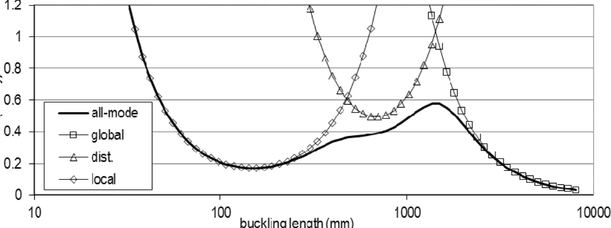
classical FSM works only on prismatic members. From the point of view of determining critical loads for G, D or L buckling, FSM is similar to FEM. However, FSM software packages, like THIN-WALL and CUFSM tried to overcome this problem by the automatic determination of the critical stress as a function of the buckling half-wavelength, which plot is frequently referred as signature curve. In case of many practical cross-sections the signature curve has two minimum points at smaller wave-lengths, while after a certain wave-length it tends asymptotically to zero (or to a small non-zero value), see Figure 1.3. By using this signature curve the G, D and L critical loads can be determined as follows: the first minimum point can be regarded as critical load for L, the second minimum point as critical load for D, while the value at the global buckling length (based on the member length and end restraints) is the critical load for G. Unfortunately, the signature curve might have more or less than two minimum points; in such cases this procedure becomes uncertain, but even in these cases the signature curve can be useful in critical load determination.

Figure 1.3: Typical signature curve and buckled cross-section shapes of a C-section member

(16)

For many years the generalized beam theory (GBT) was the only method able to directly calculate critical loads separately for G, D or L buckling. Originally it was developed to analyse global and distortional modes, then extended to local (and other) modes, too [19/1- 21/1]. First- and second-order (i.e., linear buckling) analyses are both possible, considering isotropic and various orthotropic materials [22/1-24/1]. Originally it handled simple cross- section members, then extended to very general cross-sections [25/1-28/1]. For a long time (including the time when the here-presented research has started, circa 2003) a major drawback of the method was that it lacked publicly available software implementation, which hole was later filled by the development of GBTUL software [29/1-30/1]. GBT shares most of the advantages and limitations of FSM: it elegantly handles straight prismatic members, with a relatively small number of DOF, but it is not easy (and in some cases, probably, impossible) to generalize it to more complicated cases (e.g., tapered members, members with holes, frames built up from thin-walled members, etc.). Nevertheless, GBT is probably the most researched area in thin-walled research during the last two decades, and here just a few important works are referred out of the many dozens of publications.

1.5 Modal decomposition

Two basic tasks can be identified and distinguished in the context of calculation of critical load for global-distortional-local buckling. One is the calculation of pure critical load when the aim is to calculate critical load specifically to G, D or L buckling. This could be done while forcing the member to deform in accordance with a buckling type (in other words: to constrain the deformation into a certain type). The lowest critical load from a constraint calculation could directly be used as critical load for the given buckling type.

The other task is buckling mode identification, when critical load is calculated without any preliminary restriction on the deformations (as in regular FEM or FSM calculations), but after the determination of the buckled shape it is identified, i.e., it is defined whether the given mode belongs to which class. Since general buckling modes rarely identical to any pure mode, in the practice the mode identification defines what the participations from global, distortional and local modes are in a general deformation mode. In real design situations, then, critical load for, say, distortional buckling can be estimated by the lowest critical load in which the participation of distortional deformations is dominant.

It is to note that modal identification can be applied to any deformations of a thin-walled member, however, in this dissertation it is applied only to buckled shapes obtained from a linear buckling analysis. Also, various calculations with enforced constraints can be performed (e.g., first- or second-order static analysis, dynamic analysis, etc.), however, in this dissertation only linear buckling problems are solved with constraints.

Evidently, both tasks require a clear definition of buckling classes, and require the ability of constructing deformations that satisfy the definition of a given class. When discussing these tasks in general, the whole problem will be referred here as modal decomposition. Modal decomposition has been a challenging task for a long time. The basic dilemma is that general methods, which can handle arbitrary cross-sections, boundary conditions, and loads, cannot do modal decomposition; while, specialized methods, which successfully solve buckling classification, cannot readily handle general cross-sections, boundary conditions, and loads.

The general aim of the research summarized in this dissertation is to develop numerical procedures so that modal decomposition would become available for a relatively wide range of practical situations.

(17)

1.6 Outline

This dissertation summarizes the author’s research activity on modal decomposition of thin- walled members. The dissertation focuses on those new results in which the author’s contribution has been dominant. Other closely related works, some of them with the contribution from the author, will also be mentioned for the sake of completeness.

The dissertation covers results from approx. 10 years, i.e., from the period between 2003 and 2014. It starts with the presentation of the constrained Finite Strip Method (cFSM), where the fundamental buckling classes has been defined by mechanical criteria, and the criteria are systematically implemented into the semi-analytical finite strip method. cFSM was the first shell-model-based discretization method which was able to perform modal decomposition.

The first version of cFSM was developed in 2004-05. This version handled members with pinned-pinned end restraints and open cross-section only. This original cFSM is presented in Section 2.

Later cFSM has been extended to handle other end restraints, and very recently, to handle closed cross-sections. This latter task – completed in 2012-14 – is summarized in Section 3 of this dissertation.

After development the original cFSM, modal system of base functions for the deformation- displacement field of a thin-walled member become available. The modal nature of the base system has been utilized in the (approximate) modal identification of buckling modes calculated by shell finite element analysis. The method, presented in Section 4, can be considered as the first method which provided an objective (i.e., mathematical) way to identify buckling modes calculated by shell FEM.

In validating numerical methods, comparison to analytical solution is always useful and important. Comparison of cFSM pure global results to classical analytical solutions revealed some differences. As it turned out, the differences are due to the differences between beam- model and shell-model. Therefore, shell-model-based analytical solutions for the critical loads have been worked out for a number of classical problems. In these works the thin-walled member is considered as a set of thin flat plates, constraints are introduced to enforce the member to deform in accordance to global mode (based on a certain global mode definition), from which alternative formulae for the critical loads are determined. In other words, the global modes are determined as in cFSM, but, unlike in cFSM, analytically. The analytical results are presented in Section 5.

(18)

2 Constrained Finite Strip Method for open cross- section members

2.1 Introduction

2.1.1 General

The constrained finite strip method (cFSM) is a special version of semi-analytical finite strip method (FSM), where mechanical constraints are applied to enforce the member to deform (e.g. buckle) in accordance with desired buckling modes: global, distortional, local, and other buckling. This Chapter summarizes the idea and most important derivations that are necessary for the method, following the publications [1/2-8/2]. First the FSM is briefly summarized (in Section 2.1.2). Then the constrained method is presented: the concept is outlined (Section 2.1.3), mode definitions are provided (Section 2.1.4), and some important cFSM terms are defined (Section 2.1.5). Then the constraints matrices are derived (in Sections 2.2 and 2.3). In Section 2.4 the application of the method is illustrated.

2.1.2 FSM essentials

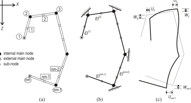
A typical open thin-walled member is given in Figure 2.1. The shaded portion is a strip (element) in an FSM mesh. Two left-handed coordinate systems are used throughout this Chapter: global and local, see Figure 2.1. The global coordinate system is denoted as: X-Y-Z, with the Y axis parallel with the longitudinal axis of the member. The local system is denoted as x-y-z, the y axis is parallel with Y, x is the in-plane transverse direction, and the z axis is perpendicular to the x-y plane. The displacement degrees of freedom (DOF) are assigned to nodal lines, that are longitudinal edge lines of the strips, and can be interpreted as amplitudes of the assumed longitudinal shape functions. Three translations (U-V-W) and a rotation () are considered as global displacements. Similarly, there are three translations (u-v-w) and a rotation () in the local system. It is to mention that the positive sign of the rotational DOF throughout Section 2 is the opposite of the positive rotation of the coordinate system (as shown in Figure 2.1), since (slightly strangely) this sign rule was used in the original work of Cheung [9/1-11/1] which later was adopted by many other FSM work e.g. [16/1-18/1] including the first cFSM publications [1/2-8/2].

Figure 2.1: FSM discretization, coordinate systems, displacements

(19)

The displacements of each strip is comprised of small deflection plate bending (w, ) and plane stress (u, v) for the membrane behaviour. Standard linear and cubic shape function are used in the transverse direction, while trigonometric functions (or function series) in the longitudinal direction. In case of pinned-pinned end restraints and longitudinal end loading, simple sine and cosine functions are appropriate as follows [9/1-11/1]:

a y m u

u b x b y x

x

u 







 



 



 



 



 

 

 1 sin

) , (

2 1

a y m v

v b x b y x

x

v 







 



 



 



 



 

 

 1 cos

) , (

2 1

a y m w

w b x b

x b

x b x x b

x b

y x x

w 





















































 











  











  

 3 2 2 3 2 sin

1 ) , (

2 2 1 2 1 2 3 3

3 2

2 2

3 2 3

3 2

2

For an individual strip the plate bending and membrane behaviour are completely uncoupled;

however, assembly of the strips into the global stiffness matrix causes coupling of membrane (in-plane) and bending (out-of-plane) behaviour any time the angle between two adjacent strips is nonzero.

It is to note that other boundary conditions may be treated but are not discussed here in Section 2. Moreover, at least two software implementations are available following these basic assumptions: THIN-WALL [13/1-15/1] and CUFSM [17/1-18/1]. The procedures presented here were implemented in CUFSM by using MatLab [9/2].

Both the elastic stiffness and geometric stiffness matrices can be assembled via the usual steps of finite element or finite strip method, see e.g. [16/1]. In case of Ke linear elastic material is considered. In case of Kg standard second-order strain terms are considered, assuming longitudinal end loads only (constant trough the thickness and linearly changing with local x axis). Once the stiffness matrices are compiled, buckling modes of a thin-walled member can be determined by solving the generalized eigen-value problem as follows:

Φ ΛK Φ

K_e  _g

where, Ke is the global elastic stiffness matrix and is a function of the member length, a,



^Φ₁ ^Φ₂ ^Φ_nDOF



Φ ... , is the matrix of eigen-vectors, where nDOF is the number of DOF (nDOF is equal to 4×n, where n is the number of nodal lines), ^^diag



^₁ ^₂ ... ^_nDOF



is the diagonal matrix of eigen-values, and Kg is the global geometric stiffness matrix. In a typical application of the FSM (for thin-walled members) Eq. (2.4) is solved for various member lengths for a given axial stress distribution, then the calculated  values are plotted against the buckling length. Note, any deformation, d (including a buckling mode, i) is described in terms of their global DOF, which include longitudinal (V) translations, transverse (U and W) translations, and rotations ().

2.1.3 Framework for constrained FSM

The primary objective of cFSM is to define constraint matrices for each of the buckling mode classes. When applied, such a constraint matrix reduces the general deformation field, which is expressed by the nDOF FSM DOF, to a smaller DOF deformation field that satisfies the criteria defined for the given class. In practice, relationship between the nodal displacements can be established in the form of:

(2.1) (2.2)

(2.3)

(2.4)

(20)

M Md R d

where d is a general nDOFelement displacement vector, dM is a displacement vector in the reduced space, and RM is the constraint matrix related to a given mode. Note, the subscript M expresses the constraint to a mode or a group of modes, i.e., M may be replaced by G (global), D (distortional), L (local), O (other) or any combination of them, e.g. GD, GDL, etc. It should also be noted that the dM vector, being in a reduced DOF space, is not necessarily associated directly with the original FSM nodal displacement DOF, but rather should be interpreted as a vector of generalized coordinates.

Application of RM, via Eq. (2.5), defines a subspace of the original FSM DOF space that meets the criteria of mode M. Thus, the columns of RM may be considered as a set of base vectors in this space of mode M. Transformation inside the space of M is also possible, and thus the base vectors defined by RM are not unique. The vector space defined by the base vectors of a given mode (included in the relevant RM) will also be referred to as the G, D, L or O space, as well as we may speak about the GD space (as a union of G and D spaces), GDL space (as a union of G, D and L spaces), etc. Naturally, the GDLO space which includes all deformations is itself identical with the original FSM DOF space.

A buckling mode shape (eigen-vector, ) is itself a deformation field, and thus the constraint of Eq. (2.5) may be employed on . By introducing Eq. (2.5) into Eq. (2.4), then pre- multiplying by RMT, we arrive at

M M g M M M M e

M K R Φ Λ R K R Φ

R ^T  ^T

which can be re-written as

M M g, M M M

e, Φ Λ K Φ

K 

which is recognizable as a new eigen-value problem, now in the constrained DOF space spanned by the given mode or modes (M). Here, Ke,M and Kg,M are the elastic and geometric stiffness matrix of the constrained FSM problem, respectively, defined as

M e M M

e R K R

K _,  ^T and K_g_,_M R_M^TK_gR_M

Note, RM is an nDOF×nM matrix, where nM is the dimension of the reduced DOF space.

Consequently, Ke,M and Kg,M are nM×nM matrices unlike Ke and Kg which are much larger nDOF ×nDOF matrices. Thus, application of the constraint represents a form of model reduction.

Finally, M is an nM×nM diagonal matrix containing the eigen-values for the given mode or modes only, and M is the matrix with the eigen-modes (or buckling modes) in its columns.

Derivation of each of the various RM matrices requires different methodologies. Some may be defined directly (e.g., RL or RO), while others require relatively long derivations (e.g., RD or RG). In some cases no other approach is known than the one used and presented below (e.g., for RD), while in other cases more than one approach exist.

2.1.4 Definition of buckling classes

The separation of global (G), distortional (D), local (L) and other (O) deformation modes are completed through implementation of the following three criteria.

Criterion #1: (a) xy = 0, i.e., there is no in-plane shear, (b) x = 0, i.e. there is no transverse strain, and (c) v is linear in x within a flat part (i.e. between two main nodes).

(2.5)

(2.6)

(2.7)

(2.8)

(21)

Criterion #2: (a) v ≠ 0, i.e., the warping displacement is not constantly equal to zero along the whole cross-section, and (b) the cross-section is in transverse equilibrium.

Criterion #3: x = 0, i.e., there is no transverse flexure.

Application of the criteria to the G, D, L, and O (global, distortional, local, and other) buckling mode classes is given in Table 2.1, defining whether the given criterion is fulfilled (Yes), not fulfilled (No), or irrelevant (). It is to observe that Criterion 1 is essentially identical to the ones widely used in theories for open thin-walled beams, also referred to as Vlasov’s hypothesis.

Table 2.1: Mode classification

G modes D modes L modes O modes

Criterion #1 – Vlasov’s hypothesis Yes Yes Yes No

Criterion #2 – Longitudinal warping Yes Yes No 

Criterion #3 – Undistorted section Yes No  

The above criteria are initiated by the generalized beam theory (GBT), which – before developing cFSM – was the only known method possessing the ability to produce and isolate solutions for all the global, distortional, and local buckling modes in a thin-walled members.

It is to emphasize, however, that the complete set of these criteria never explicitly appeared in (early) GBT publications. Indeed, GBT does not require having such complete set of criteria, since in GBT there is no pre-defined displacement field which then is separated into some practically meaningful classes, but the displacement field is built up from the selected modes where the user – based on some intuition, or preliminary studies, or previous experiences – defines the modes to consider in the analysis.

Note, for cross-sections with less than or equal to one internal main node, the mode classes slightly overlap. In the original cFSM this problem has not been properly addressed, so, such cross-sections are assumed to be excluded in Section 2 (but will be handled in Section 3).

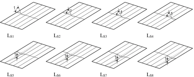
Further, O mode space may be separated into transverse extension (T) and shear (S) mode spaces (see [1/2]). Since in the original cFSM publications this separation has not been used and/or utilized, therefore, will not be addressed in Section 2, but will be discussed in detail in Section 3. Finally, Table 2.1 shows the mode classification as it is appeared and used in the original cFSM papers and software implementations; later the criteria are refined, as will be discussed in Section 3.

2.1.5 Further cFSM terminology

The line of intersection of two connecting plates will be called the nodal line (or simply:

node), while the plates themselves are referred as strips. As will be shown, it is important to distinguish between main nodes, where the two connecting strips have a non-zero angle relative to one another, and sub-nodes, where the two connecting strips are parallel. Further, main nodes are categorized as internal main nodes (also referred as corner nodes) or external main nodes (also referred as end nodes), depending on whether at least two plates or only one single plate is connected to them. (Note, sub-nodes are always internal nodes). Thus, the total number of nodes (or nodal lines) is n, consisting of nm main nodes and ns sub-nodes (nm+ns = n). Considering that the total number of nodal lines is n, and 4 displacements are assigned to each nodal line, the total number of displacement DOF is: nDOF = 4×n.

In some cases (i.e., for global and distortional modes as will be shown) sub-nodes may be eliminated. The resulting strips, i.e. the flat plates between main nodes, are called main strips.

(22)

Thus, an open cross-section thin-walled member may be described as either the assemblage of (n-1) strips, or (nm-1) main strips, whichever description is more appropriate. Note, all these terms are illustrated in Figure 2.2.

The order of the DOF in the displacement vector and in the global stiffness matrix has no theoretical importance. Nevertheless, a properly selected order makes the developed expressions simpler. For this reason we introduce here a special DOF order used throughout the sub-sequent derivations (in Chapter 2), as follows:



^V ^T ^V^T ^U ^T ^W ^T ^U ^T ^W ^T ^Θ^T



^T

d _m _s _m _m _s _s

where Vm is an nm-element partition for longitudinal translation (Y-dir.) of main nodes, Vs is an ns-element partition for longitudinal translation of sub-nodes, Um and Wm are (nm-2) element partitions for transverse translations of the internal main nodes, Us and Ws are (ns+2) element partitions for transverse translations of the external main nodes and sub-nodes,  is an (nm+ns) element partition with the rotational DOF.

2.2 Derivation for R

GD

2.2.1 Strategy

To have RG and RD, first RGD is derived, and then it is separated into RG and RD. What makes it possible and relatively convenient to follow this approach, is that as a direct consequence of the applied mode definitions, in the case of G and D modes, the member displacements (U, W,

) can be expressed as a function of the longitudinal displacements (V), i.e., global and distortional modes are completely and uniquely defined by cross-section warping. Further, the warping displacements may themselves be used to separate the G and D spaces from one another. As a consequence, (i) it is possible to develop a mathematical relationship between longitudinal displacement DOF and all the other DOF, (ii) the number of GD base vectors is equal to the number of main nodes (nm), and (iii) any set of nm independent warping distributions is applicable to serve as system of base vectors.

Thus, the main goal here is to establish the mathematical relationship between the longitudinal displacement DOF of the main nodes (Vm) and all other DOF. The relationship is set up in two steps: first the effect of Criterion #1 is considered, then, in the second step, the impact of Criterion #2 is taken into consideration.

2.2.2 Impact of Criterion #1 – unbranched cross-sections

Numbering of an open, unbranched cross-section can conveniently be handled by the system shown in Figure 2.2, where node and strip numbers appear in circles and squares, respectively.

When we consider Criterion #1, sub-nodes can (and should) be disregarded, as will become clear from the derivations. Linearity of warping within a flat element is automatically satisfied by the selection of FSM shape functions.

(2.9)

(23)

(a) nodes and strips with sub-nodes (b) nodes and strips without sub-nodes Figure 2.2: Description of an open, unbranched cross-section

The two null strain criteria can be written as:

0



 

 x

u

x and 0







 

 x

v y u

xy

By substituting Eq. (2.1) into the null transverse strain criterion we get u

u u₁ ₂ 

Furthermore, by substituting Eq. (2.2) into the null shear strain criterion, we get:

 

bkm

v v

u 1

2 1



with km = m/a. The physical meaning of Criterion #1 is illustrated in Figure 2.3 where unconstrained (left) and constrained (right) deformations are shown.

Figure 2.3: Membrane deformations of a strip: general (left) and constrained (right) Let us apply Eq. (2.12) for an open, unbranched cross-section. Let us consider the i-th main nodal line of with the connecting main strips: (i-1)-th and (i)-th. The angles of the main strips (with respect to the positive x-axis) are ^i-1) and ^i), respectively.

 

_



 



 

 _



) 1 ( 2

) 1 ( ) 1 1 ( )

1 ( )

1

( 1 1 1

i i i i

m i

v b v k b

u and

 

_



 



 

 ₍₎

2 ) ( ) 1 ( )

( )

( 1 1 1

i i i i

m i

v b v k b

u

(2.10)

(2.11)

(2.12)

(2.13)

Modal decomposition in the buckling analysis of thin-walled members