Neural Network Linearization of Pressure Force Sensor Transfer Characteristic

Neural Network Linearization of Pressure Force Sensor Transfer Characteristic

Jozef Vojtko, Irena Kováčová, Ladislav Madarász, Dobroslav Kováč

Faculty of Electrical Engineering and Informatics, Technical University of Košice, Letná 9, 042 00 Košice, Slovak Republic

Jozef.Vojtko@tuke.sk, Irena.Kovacova@tuke.sk, Ladislav.Madarasz@tuke.sk, Dobroslav.Kovac@tuke.sk

Abstract: The paper deals with an elastomagnetic sensor of pressure force and neural network design in order to achieve linear sensor output. There are described basic properties of such sensor and its equivalent electrical scheme. The feeding and evaluating circuits were designed in order to obtain the optimal working conditions.

Keywords: measurement, elastomagnetic sensor, neural network, non-linearity, hysteresis

1 Introduction

Elastomagnetic sensors have become more widespread owing to their extensive use in industrial and civil automation. However, designing low-cost and accurate sensors still requires great theoretical and experimental efforts to materials engineers. But this task can be solved by advanced electronic techniques for automatic calibration, linearization and error compensation.

2 Basic Properties of Elastomagnetic Sensor

The elastomagnetic sensor [EMS] of a pressure force that utilizes the Villary´s phenomena principle, which consists of the fact that if a ferromagnetic body is subjected to mechanical stress, its form is changed and consequently its permeability is changed, too [1]. Villary´s principle is based on equation:

ϑ ^,ϑ

, p

H H

w p

M ⎟

⎠

⎜ ⎞

⎝

⎛

∂

= ∂

⎟⎟⎠

⎜⎜ ⎞

⎝

⎛

∂

∂ (1)

where M is magnetic polarization, p is general pressure, w is relative deformation, H is intensity of magnetic field, ϑ is ambient temperature.

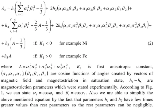
We can state magnetostriction coefficient in saturation for cubic crystal shown in Fig. 1 by following equation:

⎟+

⎟

⎠

⎞

⎜⎜

⎝

⎛ −

=

∑

= 3

2 1

3

1

1 2 i

i i

s h α β

λ 2h₂

(

α₁α₂β₁β₂⁺α₁α₃β₁β₃⁺α₃α₂β₃β₂

)

⁺

⎟+

⎟

⎠

⎞

⎜⎜

⎝

⎛ + −

+

∑

= 3

1 3

2 2

3

1

4 4 A

h _i

i i β

α

(

^{+ +} 2 3 1

)

⁺

2 3 1 3 2 2 1 3 2 2 2 1 3 2 1

2h5αα α β β α α α β β αα α β β

⎟⎠

⎜ ⎞

⎝⎛ −

+ 3

1

3 A

h if: K₁<0 for example Ni (2)

A h₃

+ if: K₁>0 for example Fe

where A=α₁²α²₂ +α₂²α₃²+α₃²α₁², K₁ is first anisotropic constant,

(

α₁,α₂,α₃

) (

, β₁,β₂,β₃

)

are cosine functions of angles created by vectors of magnetic field and magnetostriction in saturation state, h₁−h₅ are magnetostriction parameters which were stated experimentally. According to Fig.

1, we can state α_i =cosϕ_i and β_i =cosγ_i. Also we are able to simplify the above mentioned equation by the fact that parameters h1 and h2 have few times greater values than rest parameters so the rest parameters can be negligible.

Figure 1 Single cubic crystal

The resulting magnetostriction in directions <100> and <111> will be given as:

a b

γ1

[000]

z

y

x

[111]

c [xyz]

[1 ½ 0]

[abc]

ϕ1

ϕ3

ϕ2

γ

2

γ3

⎟+

⎟

⎠

⎞

⎜⎜

⎝

⎛ −

=

∑

= 3

1 2

3 ³ ₂

1

100 2 i

i i

s λ α β

λ 3λ111

(

α1α2β1β2+α1α3β1β3+α3α2β3β2

)

(3) Next relation describes dependency between magnetic induction and magnetic intensity:

( )

^H

B = μ+Δμ (4)

where Δμ represents the increment of permeability caused by acting of external pressure force. The next relation can be obtained by comparing of increments of magnetic and elastomagnetic energies:

H =σλm

μ

Δ ²

2

1 (5)

where λ_m represents a magnetostriction coefficient. It is defined like:

2 2

2 3

s s

m M

λ M

λ = (6)

It generally holds that:

s

s B

B M

M = (7)

By utilizing of the last two equations we can obtain the final dependence for permeability increment caused by the acting of external pressure force [2]:

2 2

3

s s

B μ μ= σλ

Δ (8)

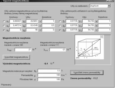
For permeability increment calculation we can utilize software calculator shown in Fig. 2. Since the permeability determines the magnetic field in a ferromagnetic body, so the magnetic field is also changed and we could measure its changes by changes of the induced electric voltage.

On the base of the above mentioned one can see that the pressductor can be described as a transformer in which the mutual inductance between the primary and secondary windings is changed proportionally to the acting stress or to the pressure, but only in the case if magnetizing current Im is constant and output current Is is negligible.

Figure 2 Intelligent calculator

The elastomagnetic sensor equivalent electrical scheme is shown in Fig. 3.

R₁ L ₁ I_p I /_s p L ₂.p² R ₂.p²

U _R1 U _L1

U _p U m L m

I m

U _s U _L2 U _R2

R m p.

Figure 3

Elastomagnetic sensor equivalent electrical scheme

The change of the output voltage value can be calculated by following equation:

( )

⋅

⋅

− ⋅

⋅ −

⋅

⋅

⋅

=

Δ 2

2

1 2 1 2

1

2 2 2

ln 2 2

4

s p s

p s

s B

r r r r

h r r I N N f

U λ μ

π π π

r F r r

B I N F fN

h

r _s

s p p

s ⋅ ⋅

=

⋅

⋅

1 2 2 2

2

2

8 ln 2

1

π μ

λ (9)

This equation corresponds with practical manufacturing of elastomagnetic sensor in Fig. 4 [3]. Properties of the ferromagnetic material have a significant influence on sensor sensitivity, mainly: saturation magnetostriction coefficient

λ

_s, permeability of material

μ

and saturation intrinsic induction

B

_s (for elastomagnetic sensor EMS-200kN:

λ

_s

= 2.15 10 ⋅

⁻⁶,

μ = 9.55 10 H/m ⋅

⁻⁴ ,

1.28T B

s

=

).

a)

b) Figure 4

Sketches of elastomagnetic sensor

a) composed sensor EMS-200kN, b) detail of sheet element

The described circuit fully corresponds to the transformer. In this case, the relation between magnetic intensity and magnetic induction is given by nonlinear hysteresis curve.

The maximum useful signal is obtained if output current Is is reduced to the minimum and if the influence of primary current Ip effective value is eliminated.

In this case, the magnetizing voltage Um corresponds to the maximum output voltage Us for given operating point which is depending on the primary current Ip

value and the acting force. Such a way can be reduced the power of the feeding source.

3 A Design of the Feeding and Evaluating Circuits

The feeding circuit must fulfill basic condition which consists in the current feeding request, because only in this case, the change of acting pressure force on the elastomagnetic sensor core will be represented by the change of output secondary voltage Us [4]. An example of such feeding source realization is shown in Fig. 5. Such a way is simply possible to secure realization of the harmonic constant current source by step down line voltage transformer with small output power.

~

+ - R R

+Ucc

-Ucc OA

Q1

Q2

Elastomagnetic Sensor

F

_Output

~

Signal DownStep

Transformer

VoltageLine

i i ref u p

i i

in out

Figure 5

An example of the optimal feeding source

For second request fulfilling, which is concerning to the secondary winding current Is minimum value we must to secure as high as possible input impedance of evaluating circuit. A simple and suitable output evaluating subcircuit can be realized by OA as it is shown in Fig. 6.

Figure 6

An example of output subcircuit connection with high impedance

4 Neural Network Design

The neural network (NN) is expected to eliminate transformer nonlinearity.

However, NN output should be linear and expressed by equation of straight line.

In order to achieve this aim, several NN models were designed. The differences between linear output and the real sensor output are shown in the Fig. 7. The characteristics ΔU_i is gained from output sensor voltage U2↑ = f(F) (if force F was increasing from 0 kN to 200 kN – characteristic upward) and characteristics ΔUd

is gained from U2↓ = f(F) (if force F was decreasing from 200 kN to 0 kN – characteristic downward). It can be expressed by next equation:

lin

i U U

U = −

Δ _2↑ (10)

lin

d U U

U = −

Δ _2↓ (11)

Figure 7

Differences between the linear and the real sensor outputs

+

+Ucc

-Ucc

OA

input output

The NN task is to reduce the deviation between U2↑, U2↓ and linear regression of sensor output Ulin. Finally, the differences ΔU_i and ΔU_d will be limited. The most common artificial neural network, called multilayer feed-forward neural network (FFNN) was used for this purpose [5]. Conception of FFNN with one-unit time delay is shown in Fig. 8.

Figure 8 The conception of NN

The sensor output is at the same time the NN input. However, in this proposal the two NN input neurons are used. The both are directly connected to sensor via ADC converter, but the second one is time delayed. A decreasing of sensor errors is expected by using this NN connection.

5 Training Process

The topology of NN consists of 10 neurons in hidden layer, which seems to be the most convenient according to computing speed and accuracy. There were 20 000 training cycles used. Like a learning algorithm the backpropagation was used and it offers an effective approach to the computation of the gradients [6], in Fig. 9.

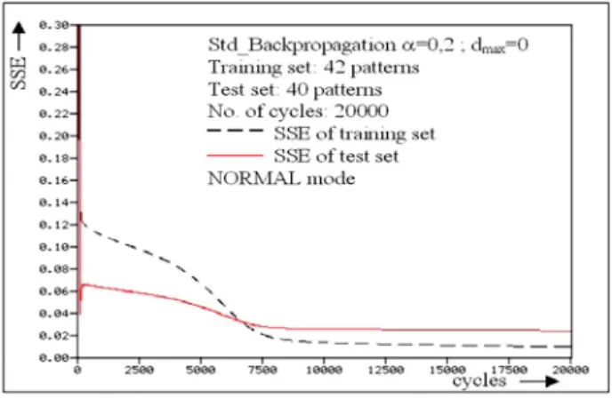
The learning parameter α, which specifies the step width of the gradient descent, was changed in the wide range (see Fig. 10). Here is the SSE (sum of square errors) dependence on training cycles. As we can see, the training process with higher learning parameter achieves smaller SSE at the constant number of training cycles.

If α parameter was more than 1, the sum square error (SSE) of training set was decreased rapidly (the NN respond to trained data was good), but SSE error of test set was increased (the NN respond to untrained data was bad) – over-trained NN.

Figure 9 The training process

Figure 10

The training process with different α parameter

The output of NN was oscillated at larger α parameter, so the stability of NN was not guaranteed. Advantages of higher NN learning rate was the decreasing of training cycles and at the same time the decreasing of SSE error of training set, but big disadvantages were: over-trained NN, bad generalization, oscillations of NN and instability of NN.

Conclusions

Such construction of elastomagnetic pressure force sensor is predetermined for hard field conditions and aggressive corroding media. Its output signal is even 1000 times greater as signal of resistance transducers and this fact enables to simplify feeding and data evaluation. Such sensors are also less sensitive against extremist electromagnetic interferences. A general construction of these sensors

can be realized with smaller costs and dimensions.

The neural network simulator SNNS v4.1 was used for simulation of designed NN. The NN should have decreased the sensor error and its output should have been a linear function. Fig. 11 shows the difference between tested data Utest and linear regression Ulin (ΔU_test = Utest - Ulin), and difference between NN model data UNN and Ulin (ΔU_NN = UNN - Ulin).

Figure 11

Differences between tested data, NN output and linear regression

The nonlinearity of sensor output was δS = 4,34% (for tested data δS = 2,69%).

The nonlinearity of designed model was δ_NN = 1,25% in comparison with a classical FFNN model (without one-unit time delay) where the nonlinearity was δ_NN = 1,53%. The finally, the designed model of error correction of elastomagnetic sensor by using FFNN (with one-unit time delay) achieves quantitatively lower linearity error in comparison with real sensor output.

Acknowledgement

The authors gratefully acknowledge the contributions of Slovak Grant Agency as project No.1/0376/2003 and Institutional project No. 4433 of Faculty of Electrical Engineering and Informatics, Technical University of Košice.

References

[1] M. Mojžiš et al.: Properties of 200 kN Force Sensor. Journal of Electrical Engineering, Vol. 50, No. 3-4, 1999 pp. 105-108

[2] M. Peťko: Obtainment of Prime Magnetisa-tion Work Values and Magnetisation Work Values by Using Approximate Functions. In Proceedings of the II Doctoral conference, TU FEI Košice, 2002, pp. 59-60 [3] M. Mojžiš, M. Orendáč, J. Vojtko: Pressure Force Sensor. In Proceedings

of the II Internal scientific conference, TU FEI Košice, 2001, pp. 19-20

[4] D. Kováč: Feeding and Evaluating Circuits for an Elastomagnetic Sensor.

Journal of Electrical Engineering, Vol. 50, No. 7-8, 1999, pp. 255-256 [5] S. Haykin: Neural Networks (A Comprehensive Foundation). Macmillan

College Publishing Company Inc., ISBN 0-02-352761-7, 1994

[6] M. Kuczmann, A. Ivanyi: A new neural-network-based scalar hysteresis model. IEEE Transactions on Magnetics, Vol. 38, 2002, pp. 857-860 [7] V. Kvasnička, Ľ. Beňušková, J. Pospíchal, I. Farkaš, P. Tiňo, V. Kráľ:

Introduction to neural networks theory (Úvod do teórie neurónových sietí, in Slovak), Iris Publisher, Bratislava, 1997

[8] A. Zell et al.: SNNS User Manual, version 4.2. University of Stuttgart, Institute for Parallel and Distributed High Performance Systems;

University of Tübingen, Since 1989