Parabolic Problems
Dissertation submitted to
The Hungarian Academy of Sciences for the degree “MTA Doktora”
Istv´ an Farag´ o
E¨otv¨os Lor´and University Budapest
2008
1 Preface 3 2 Qualitative properties of linear parabolic problems - reliable models 6
2.1 History, motivation . . . 6
2.2 Qualitative properties of the continuous models - reliable continuous models 11 2.2.1 Qualitative properties of the linear operators for the continuous models . . . 11
2.2.2 Connections between the qualitative properties . . . 14
2.2.3 Qualitative properties of the second order linear operators . . . 16
2.2.4 On necessity of the conditions . . . 18
2.3 Discrete analogs of the qualitative properties - reliable discrete models . . 19
2.3.1 Qualitative properties of discrete mesh operators . . . 19
2.3.2 Connections between the qualitative properties for the discrete op- erators . . . 21
2.3.3 Two-level discrete mesh operators . . . 23
2.3.4 Matrix maximum principles and their relations . . . 27
2.3.5 Basic conditions for the finite difference and finite element approx- imations . . . 34
2.3.6 The non-negativity preservation of the discrete heat conduction mesh operator in 1D case . . . 39
2.3.7 Non-negativity preservation for more general discrete mesh operators 48 2.4 The Crank-Nicolson scheme to the heat equation . . . 57
2.4.1 Some preliminaries for the Crank-Nicolson scheme . . . 59
2.4.2 Lower and upper bounds for C∞. . . 60
2.4.3 Maximum norm contractivity and accuracy of the Crank-Nicolson scheme . . . 65
2.4.4 Maximum norm contractivity for the modified Crank-Nicolson scheme 68 2.4.5 Numerical experiments with the modified Crank-Nicolson scheme . 73 2.5 Summary . . . 76
3 Analysis of operator splittings 77 3.1 History, motivation . . . 77
3.2 Classical operator splittings: the sequential splitting and the Strang-Marchuk splitting . . . 81
3.3 New operator splittings and their analysis . . . 87
3.3.1 Weighted sequential splitting . . . 87
3.3.2 Additive splitting . . . 90
3.3.3 Iterated splitting . . . 94
3.4 Further investigations of the operator splittings . . . 99 1
3.4.1 Operator splittings for Cauchy problems with a source function . . 99
3.4.2 Local error analysis . . . 105
3.4.3 Consistency and convergence of the operator splitting discretization methods . . . 109
3.4.4 Higher-order convergence of operator splittings . . . 117
3.5 Numerical solution of the split sub-problems . . . 123
3.5.1 Combined discretization methods . . . 123
3.5.2 Error analysis of the combined discretization methods . . . 126
3.5.3 Richardson-extrapolated sequential splitting with numerical solu- tion methods . . . 129
3.5.4 Model for a stiff problem: reaction-diffusion equation . . . 131
3.6 Air-pollution modelling - Danish Eulerian Model (DEM) . . . 134
3.6.1 Examples of splitting procedures for air pollution models . . . 135
3.6.2 Some comments on the examples . . . 137
3.6.3 Numerical results obtained by running UNI-DEM . . . 138
3.6.4 A simplified air pollution model of one air column . . . 139
3.7 Conclusion . . . 144
Bibliography 145
Appendices 157
A The Magnus method 157
B Operator splittings for non-linear operators 159 C Operators splittings for the Maxwell equations 160
Preface
Many phenomena in nature can be described by mathematical models which consist of functions of a certain number of independent variables and parameters. In particular, if some phenomenon is given by a function of spatial positions and time, then its description gives a handle to a wealth of (mathematical) models, which often consist of equations, usually containing a large variety of derivatives with respect to the variables. Apart from the spatial variable(s), which are essential in the problems to be considered, the time variable plays a special role. Indeed, many processes exhibit gradual or rapid changes as time proceeds. They are said to have an evolutionary character and an essential part of their modelling is therefore based on causality; i.e., at any time the situation is dependent of the past. Mathematical modelling of such phenomena leads to the so-called time-dependent partial differential equations, i.e., to equations that involve time t as a variable. The analysis of mathematical models of this kind is the topic of this dissertation.
Since we are not typically able to give the solution of the mathematical model in a closed (analytical) form, we construct some numerical and computer models that are useful for practical purposes. The ever-increasing advances in computer technology has enabled us to apply numerical methods to simulate plenty of physical and mechanical phenomena in science and engineering. As a result, numerical methods do not usually give the exact solution to the given problem, they can only provide approximations, getting closer and closer to the solution with each computational step. Numerical methods are generally useful only when they are implemented on computer using a computer programming language.
The study of the performance of numerical methods is called numerical analysis. This is a mathematical subject that considers estimating/controlling of the error in the process- ing of numerical methods and the subsequent re-design of the methods.
We note that applied mathematics started in the 17th century. Numerical aspects found a natural place in the analysis but the expression “numerical mathematics” did not exist at that time. However, numerical methods invented by Newton, Euler, and at a later stage by Gauss, still play an important role even today. In that time fundamental laws were formulated for various sub-domains of physics, like mechanics and hydrodynamics.
These took the form of simple looking mathematical equations. To the disappointment of the many, these equations could be solved analytically in a few special cases only. For this reason the technological development was only loosely connected with mathematics. The appearance and availability of the modern digital computer has changed this situation.
Using a computer, it is possible to gain quantitative (and later qualitative) information with detailed and realistic mathematical models and numerical methods for a multitude of phenomena and processes in physics and technology. Application of computers and
3
numerical methods has become ubiquitous. Computations are often cheaper than ex- periments; experiments can be expensive, dangerous or downright impossible. Real-life experiments can often be performed on a small scale only and that makes their results less reliable.
The present dissertation was motivated by two main objectives.
• The above modelling process of real-life phenomena real-life problem
+ physical model ⇒mathematical
model ⇒numerical model⇒computer model can qualitatively deform the models: those qualitative properties which are inherent in the original real-life process are not preserved for the other models. Therefore, the first goal is to guarantee quality preservation during all the above steps. (We note that the first and the last step in this modelling process are out of the scope of the dissertation.)
• It is almost obvious that the complexity of a model defines its tractableness: for structurally simple models, usually, it is easier to give qualitative characterization and/or define its solution. (For complex problems, in general, it is even impossible.) The operator splitting method is a powerful tool to decompose a complex time- dependent problem into a sequence of simpler sub-problems. The construction of such methods, their thorough analysis and application to different real-life problems are important issues of the applied mathematics.
The structure of the dissertation follows the above formulated aims.
The first chapter deals with the qualitative properties of linear parabolic problems. After a short overview, we analyze the qualitative properties in continuous models. Then we define the discrete analogues of the basic continuous properties. In both cases, the connections between the different basic qualitative properties are shown. We examine the two-level discretizations in detail, and review the finite difference and linear finite element schemes in different space dimensions. For the heat equation we examine the special scheme, known as the Crank-Nicolson method. We analyze its qualitative properties and we point out those exact bounds for the time-step under which the Crank-Nicolson scheme is qualitatively adequate. However, with a suitable modification of the Crank-Nicolson method we suggest a method which allows us to get rid of such a barrier.
The second chapter gives a systematic analysis of the operator splitting theory. We discuss the traditional methods and we present new results for their behaviour. We formulate some new operator splitting methods and analyze them. We investigate the error analysis of the operator splitting both in the cases where the split sub-problems are solved exactly and where we apply different numerical methods for the time integration of the split sub-problems.
The theoretical results are confirmed by several numerical (computer) results, a part of which is related to real-life applications.
The dissertation is based on the author’s several decades of work in the field of numer- ical analysis. A major part of the results has already been published. Nevertheless, the other part is still unpublished, either because it has just been submitted or because it is under preparation. The author is grateful to everyone who contributed to the achievement of the results and the preparation of the dissertation. It would be a hopeless attempt to
list all the names, therefore I only mention some of them. From my teachers my first supervisor, Igor Nikolayevich Molchanov and later L´aszl´o Cz´ach are those who have been motivating me during all my career as a mathematician. I am also grateful to those out- standing scientists with whom I had the opportunity to work as a co-author, especially Owe Axelsson, Cesar Palencia and Zahari Zlatev. However, my greatest thanks are to those young people, in whose careers I could actively participate in the beginning, and with whom I could work together, with some of them up to now. To my pride, several of them are recognized scientists not only in Hungary, but also abroad. I am glad and lucky to have such a long list that I would not be able to present it here. I do not want to mention any name because this could rightly hurt the remaining ones.
I thank ´Agnes Havasi, R´obert Horv´ath and Sergey Korotov for their assistance in the preparation of the dissertation.
My last thanks are of course to my family. It is not only this dissertation that could not have been written without them: their presence and constant assistance gave me the power to achieve the results of the dissertation.
Budapest, February 2008
Qualitative properties of linear
parabolic problems - reliable models
Time-dependent partial differential equations are involved into mathematical models of phenomena, like heat conduction or diffusion processes, reaction-diffusion problems (such as air pollution models, e.g., [157]), problems of electrodynamics ( Maxwell equations, see e.g., [138] ), option pricing models (Black-Scholes models [13, 103]), and many others arising in different fields of biology, chemistry, economy, sociology, etc. It is true that the state of the art in the solution of partial differential equations has not been advanced to the level that allows the researchers to obtain close-form analytic solutions of a large number of systems. This involves the need of using numerical approach.
When we construct mathematical and/or numerical models in order to model or solve a real-life problem, these models should have different qualitative properties, which typ- ically arise from some basic principles of the modelled phenomena. In other words, it is important to preserve characteristic properties of the original process, i.e., the models have to possess the natural equivalents of these properties. E.g., many processes, varying in time, have such properties as the monotonicity, the non-negativity preservation and the maximum principles. We will examine these qualitative properties in this part of the dissertation. We note that, even if we consider most simple problems, like the so-called heat equation, they can be viewed as a sub-problem, obtained by using the operator split- ting for a more complex reaction-diffusion-advection equation. (This is the topic of the next chapter.) Hence, for such a simple problem, the conditions of the preservation of the main qualitative properties of the continuous problem play an important role, too.
2.1 History, motivation
The classical theory of partial differential equations investigates general issues such as the analytical form, existence and uniqueness of the solutions, and also propose some methods which can produce exact solutions, see, e.g., [55, 59, 83, 124]. Qualitative inves- tigations came into being from the mid-fifties. Researchers assumed that the solution of the problem is at hand and tried to answer the questions: What kind of special properties does the solution have? What class of functions does the solution belong to? The most representative result in this field is the well-known maximum principle. A comprehensive survey of the qualitative properties of the second order linear partial differential equations can be found, e.g., in [34, 55, 110, 128, 149].
Real-life phenomena possess a number of characteristic properties. For instance, let 6
us consider the non-stationary heat conduction process in a physical body. When we increase the strength of the heat sources inside the body, and also the temperature on the boundary and the temperature in the initial state, then it is physically natural that the temperature does not have to decrease inside the body. Such a general property is called monotonicity. Clearly, when there is a certain heat source inside the body, the temperature on the boundary and the temperature in the initial state are non-negative, then the temperature inside the body is also non-negative at any fixed time. This property is callednon-negativity. Maximum principlesexpress the fact of existence of natural lower and upper bounds for the magnitude of temperature in the body. These bounds are defined by the (known) values of the temperature at the boundary, the initial state and the source.
The simplest form of them maximum principle states that, if there are no heat sources and sinks present inside the body, then the maximum temperature appears also on the boundary of the body or in the initial state.
As an illustration, we present several simple numerical examples for the source-free heat conduction problem.
In the first one we solve two-dimensional heat equation with a homogeneous boundary condition in the unit square. The material parameters are set to be constant one. We apply the finite element method with bilinear elements on a rectangular mesh with mash- spacing ∆x = 1/10 and ∆y = 1/12. For the time discretization, the so-called Crank- Nicolson method is used with a fixed time-step ∆t. A non-negative discretization of a non-negative initial function is depicted in Figure 2.1.1.
0 0.5 1
y
x
Temperature
Figure 2.1.1: Approximation of the initial function.
Let us choose the time-step ∆t = 0.1 and compute the approximation of the tem- perature at the fixed time level t = 1, i.e., at the 10-th time level. The result is shown on the left-hand side of Figure 2.1.2. The full time history of the approximation to the temperature at the fixed spatial point (1/2,1/6) on the interval [0,2.5] (i.e., during the first 25 timesteps) is displayed on the right-hand side of the same figure. We can observe that the non-negativity property of the initial temperature is not preserved. Naturally, negative values are impossible from the physical point of view, because both the initial temperature and the boundary temperature are non-negative. Moreover, the solution produces strange spurious oscillations, which are not present in the real physical process.
Thus, the time-step ∆t= 0.1 results in a qualitatively incorrect numerical solution. This observation can lead to the thought that the time-step has to be decreased.
Let us choose the time-step ∆t = 0.005 and execute the same calculations like above.
The result can be seen in Figure 2.1.3. The numerical solution seems to be qualitatively correct and we can be led to the false conclusion that small time-steps make the numerical solution better from the qualitative point of view.
−0.4
−0.2 0 0.2 0.4
y
x
Temperature
−0.2
−0.1 0 0.1 0.2 0.3
Time
Temperature
0 2.5
Figure 2.1.2: Approximation by the Crank-Nicolson method of the temperature at the 10th time level with ∆t = 0.1 and the time history of the temperature at the spatial point (1/2,1/6).
0 0.1 0.2 0.3 0.4
x Temperature y
0 0.05 0.1 0.15 0.2 0.25
Time
Temperature
0 0.125
Figure 2.1.3: Approximation by the Crank-Nicolson method of the temperature at the 10th time level with ∆t = 0.005 and the time history of the temperature at the spatial point (1/2,1/6).
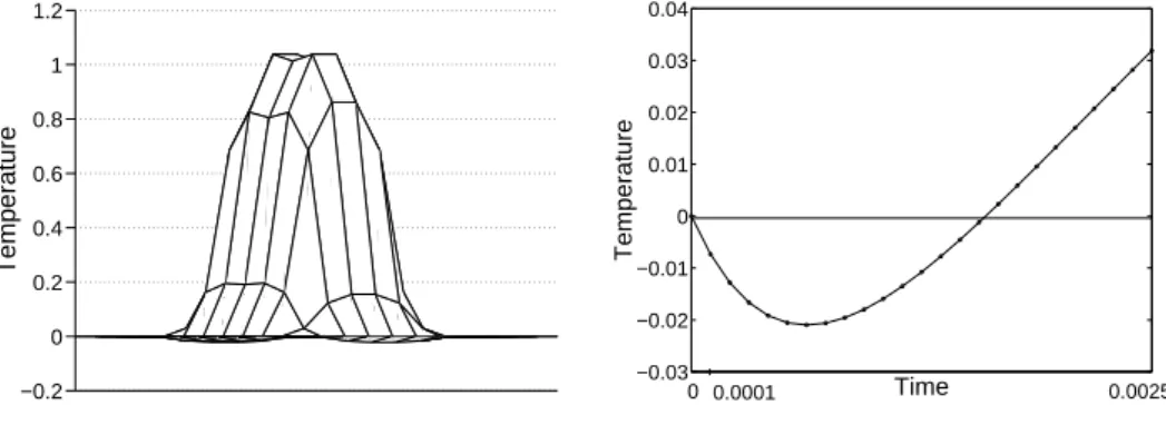
In order to demonstrate that it is not correct in general, let us choose even smaller time- step ∆t = 0.0001. The obtained result is shown in Figure 2.1.4. This numerical solution has again negative values, and it breaks the so-called maximum-minimum principle and the maximum norm contractivity property, too. This indicates that, most probably, the time-step has to be chosen within a certain interval, that is it should be neither too small, nor too large.
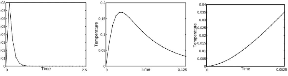
In the second numerical example, we solve the same problem with the implicit Euler method. Choosing the same time-steps, the time histories of the temperature are displayed in Figure 2.1.5. As we can see, in the case of the implicit Euler method, only small time- steps produce qualitative deficiency (negative values).
Let us turn now to the finite difference methods. We solve the problem considered above with the implicit Euler method using finite difference spatial discretization. Cal- culating with the same time-steps as in the previous two examples we obtain the time histories depicted in Figure 2.1.6. The results obtained demonstrate that there seems that no restrictions on the time-step are needed when the finite difference spatial discretization is combined with the implicit Euler time discretization.
Finally, we consider an example in three dimensions. We show that the suitable choice of the time-step is essential in this case, too. Thus, let us consider the three-dimensional heat equation in the unit cube. The material parameters are set to be constant one again.
−0.2 0 0.2 0.4 0.6 0.8 1 1.2
Temperature
−0.03
−0.02
−0.01 0 0.01 0.02 0.03 0.04
Time
Temperature
0 0.0001 0.0025
Figure 2.1.4: Approximation of the temperature at the 10th time level with ∆t = 0.0001 and the time history of the temperature at the spatial point (1/2,1/6).
0 0.02 0.04 0.06 0.08 0.1
Time
Temperature
0 2.5 0
0.05 0.1 0.15 0.2
Time
Temperature
0 0.125 −0.02
−0.01 0 0.01 0.02 0.03 0.04
Time
Temperature
0 0.0025
Figure 2.1.5: Time histories of the approximated temperature at the point (1/2,1/6)with the time-steps ∆t = 0.1, ∆t = 0.005 and ∆t = 0.0001, respectively, using the implicit Euler method and finite element spatial discretization.
The boundary points are at constant temperature zero. We apply the finite difference method with the equidistant step sizes ∆x = ∆y = ∆z = 1/10 combined with the Crank-Nicolson time discretization method. Let us suppose that an approximation of a continuous non-negative initial function is zero in every grid point except for 27 grid points in the middle of the region, where the temperature is approximated by one. The time history of the temperature at the point (4/10,4/10,4/10) using the time-step ∆t = 0.05 can be seen in Figure 2.1.7. The time-step ∆t = 0.05 results in both positive and negative temperatures, which contradicts to the non-negativity preservation property. Choosing the time-step to be ∆t= 0.003, we obtain a qualitatively adequate time history indicated on the right-hand side of Figure 2.1.7.
The above examples illustrate the fact often observed in real calculations that certain time-steps of some numerical schemes result in qualitatively adequate numerical models, while the others do not (e.g., [48, 65]). It is apparent that not only relatively large time- steps cause problems but small ones too. Moreover, unconditionally stable schemes, like the Crank-Nicolson or the implicit Euler scheme, can also produce qualitative deficiencies.
These observations rise the demand for figuring out such time-step choices that result in numerical models that mirror the characteristic nature of the original phenomenon.
The above examples show that when we construct a mathematical model of a phenom- enon, it is important to investigate whether the mathematical model (continuous/discrete) possesses the same properties as the modelled process. In the sequel we investigate the subject for the second order linear parabolic partial differential operator and for its dis- cretizations, and reveal the connections between the various qualitative properties. The results of the qualitative theory of differential equations and their discrete analogues,
0 0.01 0.02 0.03 0.04 0.05 0.06 0.07 0.08
Time
Temperature
0 2.5 0
0.05 0.1 0.15 0.2
Time
Temperature
0 0.125 0
0.005 0.01 0.015 0.02 0.025 0.03 0.035 0.04
Time
Temperature
0 0.0025
Figure 2.1.6: Time histories of the temperature at the point (1/2,1/6)with the time-steps
∆t= 0.1, ∆t = 0.005 and ∆t= 0.0001, respectively, using the implicit Euler method and finite difference spatial discretization.
−0.5 0 0.5 1
Time
Temperature
0 0.05 1.25
0 0.2 0.4 0.6 0.8 1
Time
Temperature
0 0.003 0.075
Figure 2.1.7: Time history of the temperature at the point (4/10,4/10,4/10) using the time-steps ∆t= 0.05and ∆t= 0.003, respectively.
albeit they have the importance on their own, help us to show that the qualitative prop- erties of a mathematical model correspond to the qualitative properties of the modelled phenomenon.
The discrete version of the maximum-minimum principle is commonly called the dis- crete maximum-minimum principle (or DMP in short). The topic of construction and preserving the validity of various discrete maximum principles arose already 40 years ago and was first investigated for elliptic problems (see, e.g., [23, 24, 77, 118]). Sufficient con- ditions for the validity of the DMP were given in [144] in terms of the matrix appearing in the finite difference discretization. Recently, this question for the elliptic problems is intensively investigated in many works, see, e.g., [77, 81, 125, 146]. The paper [76] inves- tigates nonlinear problems. The discrete maximum principle is generally guaranteed by some geometrical conditions for the meshes. The discrete maximum principle for parabolic problems was originally discussed discussed about 25 years ago, see, e.g., [57, 83, 131].
In [57], based on the acuteness of the tetrahedral meshes, a sufficient condition of the DMP was obtained for the Galerkin finite element solution of certain parabolic problems, including both the lumped and the non-lumped approaches. The lumped mass method and some hyperbolic prolems are considered in [10]. Actually this topic is considered in the works [36, 46, 47, 48]. In paper [46], a necessary and sufficient condition of the DMP was derived for Galerkin finite element methods and sufficient conditions were given for hybrid meshes. A comprehensive survey on DMPs can be found in papers [18, 19].
The conditions of thediscrete non-negativity preservationwas discussed in [43, 64] for linear finite elements in one, two and three dimensions, and in [38] in one dimensional case with the combination of the finite difference and finite element methods. The discrete non-negativity preservation is investigated for nonlinear problems in [145].
The discrete maximum norm contractivitywas analyzed for one-dimensional parabolic problems in [69, 80, 131, 132]. In the papers [69, 80] the necessary and sufficient condi- tions were given. In the first one, the dependence on the spatial discretization was also discussed. In the papers [131, 132] sufficient conditions were given.
For one-dimensional problems, we can deduce some other remarkable qualitative prop- erties such as the preservation of the shape and the monotonicity of the initial function, and the sign-stability (see, e.g., [52, 70, 71, 72, 107]).
2.2 Qualitative properties of the continuous models - reliable continuous models
In this part we define the main qualitative properties for the continuous models, namely, the maximum-minimum principle, the monotonicity, and the maximum norm contractiv- ity. First we consider the general setting, then we analyze the second order linear partial differential operator. We also demonstrate various interrelations between these properties.
Let Ω denote a bounded, simply connected domain in IRd (d∈IN+) with a Lipschitz- continuous boundary ∂Ω. We introduce the following sets
Qτ = Ω×(0, τ), Q¯τ = ¯Ω×[0, τ], Qτ¯ = Ω×(0, τ], Γτ = (∂Ω×[0, τ])∪(Ω× {0}) for any arbitrary positive number τ. The set Γτ is usually called parabolic boundary. For some fixed number T > 0, we consider the linear partial differential operator
L≡ ∂
∂t− X
0≤|ς|≤δ
aς ∂|ς|
∂ς1x1. . . ∂ςdxd ≡ ∂
∂t− X
0≤|ς|≤δ
aςDς, (2.2.1) where δ is the order of the operator,ς1, . . . , ςd denote non-negative integers, |ς|is defined as |ς| = ς1 +· · ·+ςd for the multi-index ς = (ς1, . . . , ςd), and the coefficient functions aς :QT → IR are bounded in the setQT. For the sake of simplicity, in what follows, the coefficient function a(0,...,0) will be simply denoted by a0. We define the domain of the operator L, denoted by domL, as the space of functions v ∈ C( ¯QT), for which all the partial derivativesDςv (0<|ς| ≤δ) and∂v/∂texist inQT and they are bounded. It can be seen easily thatLv is bounded inQ¯t? for eachv ∈domL andt? ∈(0, T), which means that infQt?¯ Lv and supQ¯t?Lv are finite values.
2.2.1 Qualitative properties of the linear operators for the con- tinuous models
Operator (2.2.1) appears in the mathematical models of many physical phenomena ([73, 82]). In these phenomena, the following quantities, often calledinput data, can be observed and measured, and hence they are supposed to be known (or easily computable):
• the values of the unknown investigated physical quantities on the parabolic boundary of the solution domain,
• the source density of the quantities inside the solution domain.
Our task is to determine the physical quantities inside the given domain. It can be usually observed in practice that the increase of the input data implies the increase of the quantities inside the solution domain for the physical phenomena described by (2.2.1).
In the mathematical models of the physical phenomena, the function v ∈ domL describes the values of the physical quantity in the domain ¯QT, that is the dependence of the quantity on place and time. The above mentioned physical property can be connected by the following definition.
Definition 2.2.1 Operator (2.2.1)is said to be monotone if for allt? ∈(0, T)andv1, v2 ∈ domL such that v1|Γt? ≥ v2|Γt? and (Lv1)|Q¯t? ≥ (Lv2)|Q¯t?, the relation v1|Q¯t? ≥ v2|Q¯t?
holds.1
Clearly, the monotonicity property of the linear operator (2.2.1) is equivalent (due to its linearity) to the widely used non-negativity preservation property.
Definition 2.2.2 The operator L is called non-negativity preserving (NP) when for any v ∈ domL and t? ∈ (0, T) such that v|Γt? ≥ 0 and (Lv)|Q¯t? ≥ 0, the relation v|Qt?¯ ≥ 0 holds.
The physical quantities inside the solution domain can be obtained by computation of the function v with given initial data. Often we may need only certain characterization ofv, which does not require the knowledge of v in the whole domain. It is typical that we are interested in range(v) over ¯QT. From the practical point of view, only such estimates are suitable which include only the known initial data. This kind of estimations is called maximum-minimum principles.
For different operators different maximum-minimum principles are valid. These are widely used in literature, because they well characterize the operator L itself (cf. [34, 55, 83, 110, 124, 128] and references therein). Now we list four possible variants of the maximum-minimum principles.
Definition 2.2.3 We say that the operatorLsatisfies the weak maximum-minimum prin- ciple (WMP) if for any function v ∈domL and any t? ∈(0, T) the inequalities
min{0,min
Γt?
v}+t?·min{0,inf
Q¯t?
Lv} ≤min
Q¯t?
v ≤max
Q¯t?
v ≤max{0,max
Γt?
v}+t?·max{0,sup
Qt?¯
Lv}
(2.2.2) are valid.
Definition 2.2.4 We say that the operator L satisfies the strong maximum-minimum principle (SMP) if for any function v ∈domL and any t? ∈(0, T) the inequalities
minΓt?
v+t?·min{0,inf
Q¯t?
Lv} ≤min
Q¯t? v ≤max
Q¯t? v ≤max
Γt?
v+t?·max{0,sup
Q¯t?
Lv} (2.2.3) are satisfied.
When the sign of Lv is known, then it is possible that the estimates involve only the known values ofv on the parabolic boundary. These types of maximum-minimum princi- ples are called boundary maximum-minimum principles. (Boundary maximum-minimum principles are frequently used in proofs of the uniqueness theorems.)
1This property is also known as the comparion principle.
Definition 2.2.5 We say that the operator L satisfies the weak boundary maximum- minimum principle (WBMP) if for any function v ∈ domL and any t? ∈ (0, T) such that Lv|Q¯t? ≥0 the inequalityies
min{0,min
Γt?
v} ≤min
Q¯t?
v ≤max
Q¯t?
v ≤max{0,max
Γt?
v} (2.2.4)
hold.
Definition 2.2.6 We say that the operator L satisfies the strong boundary maximum- minimum principle (SBMP) if for any function v ∈domL and any t? ∈(0, T) such that Lv|Q¯t? ≥0 the realtions
minΓt?
v = min
Q¯t? v ≤max
Q¯t? v = max
Γt?
v (2.2.5)
hold.
Remark 2.2.7 To show the validity of the relations (2.2.4) and (2.2.5), it is enough to show only one relation in each of them: the relation either for the minimum or for the maximum. This is true, because v ∈domL implies −v ∈ domL and the maximum of a real valued functionv is minus one times the minimum of−v, we obtain that if an operator L satisfies the WBMP, then Lv|Q¯t? ≤0 implies max{0,maxΓt?v} ≥ maxQ¯t?v. Similarly, if an operator L satisfies the SBMP, then maxΓt?v = maxQ¯t?v whenever Lv|Qt?¯ ≤0.
Although the left-hand side inequalities in (2.2.2) and (2.2.3) also imply the inequalities on the right-hand side, for practical reasons, we wrote out both the upper and the lower estimates for the function v.
The WMP and the SMP generally do not disclose the place of the maximum or min- imum values of v. The WBMP (resp. SBMP) implies that the non-negative maximum (resp. maximum) and the non-positive minimum (resp. minimum) taken over the set ¯Qt? of the functions v ∈ domL for which Lv|Q¯t? ≤ 0 (or Lv|Q¯t? ≥ 0), can be found also on the parabolic boundary Γt?.
Remark 2.2.8 We could pose the natural question of whether it is possible to define another maximum-minimum principle that is somewhat stronger than the SMP. This could be done in the form
minΓt?
v+t?·inf
Q¯t?
Lv ≤min
Q¯t?
v ≤max
Q¯t?
v ≤max
Γt?
v+t?·sup
Q¯t?
Lv, (2.2.6)
i.e., without the zero values in (2.2.3). It is easy to see that there is no sense in defining such a maximum-minimum principle because the simplest one-dimensional heat conduc- tion operator
L= ∂
∂t − ∂2
∂x2
on QT ≡ (0, π)×(0, T) does not possess this property. To show this, let us consider the function v(x, t) = e−t(sinx−2)∈domL, for which
(Lv)(x, t) = ∂v
∂t(x, t)− ∂2v
∂x2(x, t) = 2e−t. For a fixed t? ∈(0, T), we have
minΓt?
v+t?·inf
Qt?¯
Lv =−2 + 2t?e−t? >−2.
On the other hand, we have minQ¯t?
v = µ
min[0,π](sinx−2)
·(max
[0,t?]e−t) = −2,
which shows the uselessness of such a definition. The explanation of this phenomena is the following. The different maximum principles based on the comparison of the unknown solution with a function, about which we a priori know that it takes bigger values on the parabolic boundary. Then we use the monotonicity property. (We investigate the relation between the different qualitative properties in the next section in more details.) If we choose
v1 = min{0,min
Γt
v}+t·min{0,inf
Q¯t
Lv},
which stands on the left side of (2.2.2) at t = t?, and v2 = v, then the conditions of the monotonicity in Definition 2.2.1 are valid. However, with the choice
v1 = min{0,min
Γt
v}+t·inf
Qt¯
Lv it is not true anymore.
The maximum-minimum principles are in close connection with the maximum norm contractivity, which can be formulated as follows.
Definition 2.2.9 The operator L is called contractive in the maximum norm (MNC) if for any two functions v,ˆ v˜ ∈ domL and any t? ∈ (0, T) such that Lˆv|Q¯t? = L˜v|Q¯t? and ˆ
v|∂Ω×[0,t?]= ˜v|∂Ω×[0,t?], the property
maxx∈Ω¯ |ˆv(x, t?)−v(x, t˜ ?)| ≤max
x∈Ω¯ |ˆv(x,0)−v˜(x,0)|
is valid.
2.2.2 Connections between the qualitative properties
In the next theorem, the logical implications between the qualitative properties defined in Section 2.2.1 are proved. In order to see the analogy between the qualitative properties of operator (2.2.1) and its discrete versions, the conditions of the theorem are formulated for the function L1, where 1 : (x, t) 7→ 1 is the identically one function. Naturally, for operator (2.2.1), L1=−a0.
Theorem 2.2.10 The implications between the qualitative properties are shown in Figure 2.2.1. The solid arrows mean the implications without any additional condition, while the dashed ones are true under the indicated assumptions on the sign of a0.
Proof.
Implications I and II: These implications follow from the relations min{0,minΓt?v} ≤ minΓt?v and max{0,maxΓt? v} ≥maxΓt? v.
Implication III: Due to the inclusion Γt? ⊂Q¯t?, the trivial relation minΓt? v ≥minQ¯t?v holds. The reverse relation follows from the left-hand side relation of (2.2.3) and the non- negativity ofLv in Q¯t?.
Implication IV: For functions v with Lv|Qt?¯ ≥0, the left-hand side relation of (2.2.2) ensures the required relation (2.2.4).
S M P
S B M P W M P
W B M P N P M N C
L 1 > 0
I
I I I I I
I V
V V I
V I I
V I I I
L 1 > 0
L 1 = 0
Figure 2.2.1: Implications between the qualitative properties.
Implication V: This statement is a direct consequence of the definition of the WBMP.
Implication VI: Let ˆv and ˜v ∈domL be two arbitrary functions withLˆv|Q¯t? =L˜v|Q¯t?
and ˆv|∂Ω×[0,t?] = ˜v|∂Ω×[0,t?]. We consider the functions v± = ζ ± (ˆv − v˜) with ζ = maxx∈Ω¯ |ˆv(x,0)−v(x,˜ 0)|. For these functions, in view of the non-positivity of a0 and non-negativity of ζ, the estimations Lv±|Q¯t? = (−a0ζ)|Q¯t? ≥ 0 and minΓt?v± ≥ 0 are true, which implies the non-negativity of v± onQ¯t?. Thus, we have
maxx∈Ω¯ |ˆv(x, t?)−˜v(x, t?)| ≤max
x∈Ω¯ |ˆv(x,0)−v(x,˜ 0)|.
Implication VII: We suppose thata0 ≤0. We choose an arbitrary functionv ∈domL and apply the operator Lto the function ¯v =v−min{0,minΓt?v} −t·min{0,infQ¯t?Lv}.
Clearly, ¯v|Γt? ≥0. Moreover, we obtain that L¯v|Q¯t? = (Lv−min{0,inf
Q¯t?
Lv}+a0·min{0,min
Γt?
v}+a0·t·min{0,inf
Qt?¯
Lv})|Q¯t? ≥0, which implies that ¯v is non-negative on Q¯t? by virtue of the non-negativity preservation assumption. Thus
min{0,min
Γt? v}+t?·min{0,inf
Qt?¯
Lv} ≤min{0,min
Γt? v}+t·min{0,inf
Q¯t?
Lv} ≤v(x, t) for all x∈Ω and¯ t ∈[0, t?].
Implication VIII: We suppose thata0 = 0. We choose an arbitrary functionv ∈domL and apply the operatorL to the function ¯v =v−minΓt? v−t·min{0,infQ¯t?Lv}. Clearly,
¯
v|Γt? ≥0. Moreover, we obtain that
L¯v|Q¯t? = (Lv−min{0,inf
Qt?¯
Lv})|Q¯t? ≥0,
which implies that ¯v is non-negative on Q¯t? by virtue of the non-negativity preservation assumption. Thus
minΓt?
v +t?·min{0,inf
Qt?¯
Lv} ≤min
Γt?
v+t·min{0,inf
Q¯t?
Lv} ≤v(x, t) for all x∈Ω and¯ t ∈[0, t?].
An important and direct consequence of the above theorem can be formulated for non-negativity preserving operators as follows.
Theorem 2.2.11 For a non-negativity preserving operator (2.2.1)with a0 ≤0, the weak maximum-minimum principles and the maximum norm contractivity properties are also satisfied. If, in addition a0 = 0, then the non-negativity preserving operator possesses all the other defined qualitative properties.
2.2.3 Qualitative properties of the second order linear operators
The second order linear operators (i.e., δ = 2) of the form (2.2.1) have a great practical importance. Such a type of operators appears in parabolic partial differential equations, which serve as mathematical models of several important real-life problems such as heat conduction, advection-diffusion, option pricing, etc. Based on the results of the previous section, we investigate qualitative properties of the following operator
L≡ ∂
∂t − Xd
m,k=1
am,k
∂2
∂xm∂xk − Xd
m=1
am
∂
∂xm −a0, (2.2.7) where the coefficient functions and domL are defined as before (cf. introduction of this Section). The maximum principle for some special case is investigated e.g., in [34, 35, 83, 110, 128]. Let S(x, t) be the matrix of the coefficients of the second derivative terms at the point (x, t), i.e.,
S(x, t) := [am,k(x, t)]dm,k=1. (2.2.8) A sufficient condition for the operator (2.2.7) being non-negativity preserving can be formulated as follows. (We note that, with a similar approach, analogical results are proved for some more special cases in [83] and [35].)
Theorem 2.2.12 Assume that the matrix S(x, t) is positive semi-definite at each point of QT. Then the operator (2.2.7) is non-negativity preserving.
Proof. First we prove a lower estimation for the functions v ∈ domL, which will show the non-negativity preservation of the operator immediately. Thus, let v ∈ domL an arbitrary fixed function. Then the function
ˆ
v(x, t)≡v(x, t)e−λt (2.2.9)
also belongs to domL for any real parameter λ. Expressing v from (2.2.9) and applying operator (2.2.7) to it, we get
Lv =L(eλtv) =ˆ eλt
"
∂vˆ
∂t − Xd
m,k=1
am,k
∂2ˆv
∂xm∂xk − Xd
m=1
am
∂vˆ
∂xm + (λ−a0)ˆv
#
. (2.2.10) Let us fix the parameter t? ∈ (0, T). Since ˆv is a continuous function on ¯Qt?, its minimum exists on ¯Qt? and it is taken at some point (x0, t0)∈Q¯t?.
• First we assume that this point belongs to the parabolic boundary, i.e., (x0, t0)∈Γt?. Then, due to the obvious relation
ˆ
v(x, t)≥vˆ(x0, t0) = min
Γt?
ˆ v for all (x, t)∈Q¯t?, we get the estimation
infQ¯t?
ˆ
v ≥min
Γt?
ˆ
v. (2.2.11)
• Assume now that (x0, t0)∈Q¯t?. Then we get the relations
∂vˆ
∂t(x0, t0)≤0, ∂ˆv
∂xm(x0, t0) = 0, (2.2.12) and, because (x0, t0) is a minimum point, the second derivative matrix
V(xˆ 0, t0) :=
· ∂2vˆ
∂xm∂xk(x0, t0)
¸d
m,k=1
is positive semi-definite.
Let us denote by S(x0, t0)◦V(xˆ 0, t0)∈IRd×d the Hadamard product h
S(x0, t0)◦V(xˆ 0, t0) i
m,k =am,k(x0, t0)· ∂2vˆ
∂xm∂xk(x0, t0). (2.2.13) Due to the assumptions, both the matricesS(x0, t0) and ˆV(x0, t0) are positive semi- definite, hence, according to the Schur theorem (e.g., Theorem 7.5.3 in [68]), the matrix S(x0, t0)◦V(xˆ 0, t0) is also positive semi-definite.
We investigate (2.2.10) in the rearranged form e−λtLv+
Xd
m=1
am ∂ˆv
∂xm −(λ−a0)ˆv = ∂ˆv
∂t − Xd
m,k=1
am,k ∂2vˆ
∂xm∂xk. (2.2.14) Using the notation e= [1,1, . . . ,1]>∈IRd, the relation
Xd
m,k=1
am,k(x0, t0) ∂2vˆ
∂xm∂xk(x0, t0) = ((S(x0, t0)◦V(xˆ 0, t0))e,e)≥0. (2.2.15) is valid. On the base of (2.2.12) and (2.2.15), the right-hand side of (2.2.14) is nonpositive at the point (x0, t0). Hence, the inequality
e−λt0(Lv)(x0, t0)−(λ−a0(x0, t0))ˆv(x0, t0)≤0 (2.2.16) holds. Let us introduce the notations ainf := infQT a0 and asup := supQTa0, which are well-defined because of the boundedness of the coefficient function a0. For any λ > asup, we have
ˆ
v(x0, t0)≥ e−λt0(Lv)(x0, t0)
λ−a0(x0, t0) ≥ e−λt0(Lv)(x0, t0) λ−ainf ≥
≥ 1 λ−ainf inf
Q¯t?
(e−λt(Lv)(x, t)).
(2.2.17)
Since the function ˆv takes its minimum at the point (x0, t0), therefore estimation (2.2.17) implies the inequality
infQt?¯
ˆ
v ≥ 1
λ−ainf inf
Q¯t?
(e−λt(Lv)(x, t)). (2.2.18)
Clearly, the estimates of the two different cases, namely (2.2.11) and (2.2.18) together, imply that
inf¯
Qt?ˆv ≥min{inf
Γt?
ˆ
v; 1
λ−ainf inf
Qt?¯
¡e−λt(Lv)(x, t)¢
}. (2.2.19)
From (2.2.19) and from the definition of the function ˆv in (2.2.9), we obtain that v(x, t?)≥ sup
λ>asup
½
eλt?min
½ minΓt?
(ve−λt), 1 λ−ainf inf
Q¯t?
(e−λt(Lv)(x, t))
¾¾
. (2.2.20) The statement of the theorem follows from the definition of the non-negativity preservation and the estimation (2.2.20).
Remark 2.2.13 Let us consider the d-dimensional heat conduction operator L≡ ∂
∂t − Xd
m=1
∂2
∂x2m. (2.2.21)
In this case S(x, t) =I, whereI denotes thed×d unit matrix, which is obviously positive definite. Thus, for this operator the NP property holds and, according to Theorem 2.2.11, if a0 = 0 it satisfies all the above discussed qualitative properties.
For the more general operator,
L≡ ∂
∂t− Xd
m=1
∂
∂xm
(km(x, t) ∂
∂xm
)−a0(x, t) (2.2.22) the condition of the positive semi-definitness reads, obviously, as
km(x, t)≥0 for all (x, t)∈QT and m = 1,2, . . . , d. (2.2.23)
2.2.4 On necessity of the conditions
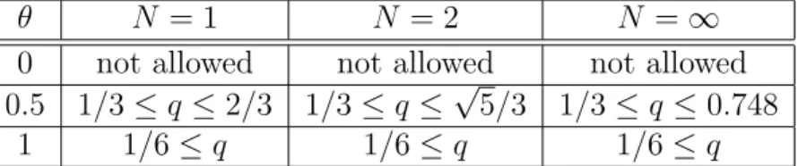
In this section we show that certain implications in Theorem 2.2.10 are strong in the sense that they cannot be reversed or sharpened. Namely, let us investigate whether the condition −a0 = L1 ≥ 0 can be changed to −a0 = L1 ≥ γ, with some constant γ 6= 0 such that the implications indicated in Figure 2.2.1 remain valid.
Theorem 2.2.14 The infimum of those values γ for which Implications VI and VII in Theorem 2.2.10 are valid, under the condition −a0 =L1 ≥γ, is zero. Similarly, for the Implication VIII the given condition of is also necessary in the same sense.
Proof. Let γ be an arbitrary negative number (i.e., a0 ≡ −γ > 0) and we consider the one-dimensional operator
L≡ ∂
∂t +γ 2
∂2
∂x2 +γ, (2.2.24)
where domLis defined similarly as for operator (2.2.1) andQT = (0, π)×(0, T). Naturally, based on Theorem 2.2.12, operator (2.2.24) is non-negativity preserving as a11=−γ/2>
0. Moreover L1 =γ =−a0 and hence a0 >0 .
We show that operator (2.2.24) does not possess the WMP and the MNC. Let us choose the function v(x, t) = (−γ/2)e−γt/2sinx, for which function the relation Lv(x, t) = 0 is true. Thus, we have
−γ
2e−γt?/2 = max
Q¯t?
v >max{0,max
Γt?
v}+t?·max{0,sup
Q¯t?
Lv}=−γ 2
for any t? ∈(0, T). This shows that the WMP does not hold for the operator defined by (2.2.24). Due to Implication I, the SMP cannot be valid, either. Let us set ˆv = v and
˜
v = 0. The relations Lˆv|Qt?¯ =L˜v|Qt?¯ = 0 and ˆv|∂Ω×[0,t?] = ˜v|∂Ω×[0,t?] = 0 obviously hold for these functions and we have
−γ
2e−γt?/2 = max
x∈Ω¯ |ˆv(x, t?)−v˜(x, t?)|>max
x∈Ω¯ |ˆv(x,0)−v(x,˜ 0)|=−γ 2. This shows that the operator (2.2.24) does not have the MNC property.
Now let γ be an arbitrary positive number and consider the non-negativity preserving operator
L≡ ∂
∂t −γ 2
∂2
∂x2 +γ. (2.2.25)
We set v(x, t) = 0.5γe−γt/2(sinx−2) and QT = (0, π)×(0, T), for which Lv(x, t) = 0.5γ2e−γt/2(sinx−1)≤0. For this function v, we get the relation
maxQ¯t?
v =−γ
2e−γt?/2 >max{−γe−γt?/2,−γ/2}= max
Γt?
v = max
Γt?
v+t?·max{0,sup
Q¯t?
Lv}
for anyt? ∈(0, T), showing that the SMP is not satisfied in this case. This completes the proof.
Remark 2.2.15 The operator (2.2.24)with the functionv(x, t) = a0ea0tsinxalso demon- strates that Implication V cannot be reversed for a0 > 0. Namely, max{0,maxΓt?v} = a0 < a0ea0t? = maxQ¯t? v. Similarly, operator (2.2.25)and the functionv(x, t) =−a0ea0t(sinx−
2) show that Implications I and II are not reversible, provided a0 6= 0.
Finally, we note that a more general setting of the problem and other counterexamples can be found in [49].
2.3 Discrete analogs of the qualitative properties - reliable discrete models
In this part we present the natural discrete analogs of the qualitative properties formulated in Section 2.2 for the continuous models.
2.3.1 Qualitative properties of discrete mesh operators
Let us assume that the sets P = {x1,x2, . . . ,xN} and P∂ = {xN+1,xN+2, . . . ,xN+N∂} consist of different vertices in Ω and on ∂Ω, respectively. (The bounded domain Ω and its boundary∂Ω were defined in Section 2.2.)
We set ¯N =N +N∂ and ¯P =P ∪ P∂. Let T and ∆t < T be two arbitrary positive numbers. Moreover, let us suppose that the natural number M satisfies the condition M∆t ≤T <(M+ 1)∆t and introduce the setR ={tn =n∆t|n= 0,1, . . . , M}. For any values τ from the set R we introduce the notations
Rτ ={t∈ R |0< t < τ}, R¯τ ={t∈ R |0< t≤τ}, R0¯τ ={t∈ R |0≤t≤τ},
(2.3.1) and the sets
Qτ =P × Rτ, Q¯τ = ¯P × R0τ¯, Q¯τ =P × Rτ¯, Gτ = (P∂× R0τ¯)∪(P × {0}).