OpenCL
György Kovács
OpenCL
György Kovács
Copyright © 2013 Typotex
Table of Contents
1. Introduction ... 1
1. The history of OpenCL ... 1
2. The present and future of OpenCL ... 6
3. OpenCL and Flynn-classes ... 6
4. What is OpenCL used for? ... 7
5. About the book ... 9
5.1. The aim and use of the book ... 9
5.2. What is the book based on? ... 9
5.3. Hardware environment ... 9
2. My first OpenCL program ... 10
1. Programming environment ... 10
2. Hello world ... 11
3. Compile, link, run ... 15
4. Summary ... 16
3. The OpenCL model ... 17
1. The OpenCL specification ... 17
1.1. Platform model ... 17
1.2. Execution model ... 18
1.2.1. Indexranges and subproblems ... 18
1.2.2. Kernel, workitem, workgroup ... 18
1.2.3. Global, workgroup and local indices ... 18
1.2.4. Context object ... 20
1.2.5. Command queue object ... 20
1.3. Memory model ... 20
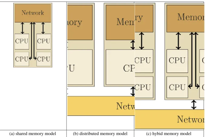
1.3.1. Classical memory models ... 20
1.3.2. The memory model of the abstract OpenCL device ... 22
1.4. Programming model ... 24
2. Summary ... 25
3. Excercises ... 25
4. The OpenCL API ... 26
1. Error handling ... 26
2. Retain/Release ... 27
3. Naming conventions ... 28
4. Platform layer ... 28
4.1. Identification of platforms ... 29
4.2. Devices, subdevices ... 32
4.3. Context ... 41
5. Runtime layer ... 46
5.1. Command queue ... 46
5.2. Event objects ... 47
5.3. Buffer objects and memory handling ... 49
5.3.1. Creation and filling of buffer objects ... 50
5.3.2. Reading and writing of buffer objects ... 53
5.3.3. Map/Unmap ... 57
5.3.4. Other memory handling functions ... 61
5.4. Synchronization ... 62
5.4.1. Event based synchronization ... 62
5.4.2. Command queue base synchronization ... 63
5.4.3. Synchronization commands ... 64
5.5. Program objects ... 66
5.5.1. Creating program objects ... 66
5.5.2. Compilation, linking ... 68
5.6. Kernel objects ... 84
5.7. Execution of kernels ... 89
5.7.1. Data parallelization ... 90
5.7.2. Functional parallelization ... 93
5.7.3. Execution of native kernels ... 95
6. Summary ... 98
7. Excercises ... 99
5. The OpenCL C language ... 100
1. The OpenCL C programming language ... 100
2. Data types ... 100
2.1. Atomic data types ... 100
2.2. Vector data types ... 100
2.3. Conversion ... 102
3. Expressions ... 104
3.1. Arithmetic conversion ... 104
3.2. Operators ... 104
3.2.1. Arithmetic operators ... 104
3.2.2. Comparison and logical operators ... 104
3.2.3. Other operators ... 104
4. Qualifiers ... 105
5. Control statements ... 108
6. Built-in functions ... 109
6.1. Workitem functions ... 109
6.2. Mathematical functions ... 110
6.3. Geometrical functions ... 113
6.4. Relational functions ... 113
6.5. Functions related to the loading and storage of vector values ... 114
6.6. Synchronization functions ... 115
6.7. Async copies from global to local memory, local to global memory and prefetch 116 6.8. Atomic functions ... 118
6.9. printf ... 119
7. Summary ... 120
8. Excercises ... 120
6. Case study - Linear Algebra - Matrix multiplication ... 121
1. Mathematical background ... 121
2. Measuring the runtime ... 123
3. CPU implementation ... 124
4. Naive OpenCL implementation ... 126
5. OpenCL C optimization ... 132
6. Increasing the granularity of the parallelization ... 133
7. The utilization of private memory ... 135
8. The utilization of the local memory ... 136
9. Summary ... 138
10. Exercises ... 138
7. Case study - Digital image processing - Convolution filter ... 141
1. Theoretical background ... 141
2. CPU implementation ... 145
3. Naive OpenCL implementation ... 148
4. Simple C optimization ... 151
5. The utilization of constant memory ... 152
6. Utilization of the local memory ... 153
7. Summary ... 157
8. Exercises ... 158
8. Image and sampler objects ... 160
1. Image objects ... 161
1.1. Instantiation ... 161
1.2. Reading/writing and filling image objects ... 166
1.3. Other functions ... 169
2. Sampler objects ... 170
3. OpenCL C ... 172
3.1. Types ... 172
3.2. Qualifiers ... 172
3.3. Instantiation ... 173
3.4. Functions ... 173
3.4.1. Reading and writing ... 173
3.4.2. Other functions ... 176
4. Example ... 177
5. OpenCL 1.1 ... 181
6. Summary ... 186
7. Exercises ... 186
9. Case study - Statistics - Histograms ... 188
1. Theoretical background ... 188
1.1. The concept of histograms ... 188
1.2. Applications of histograms ... 189
1.2.1. Histogram equalization ... 189
1.3. Adaptive thresholding ... 192
2. Histogram computation on CPU ... 193
3. Naive OpenCL implementation ... 195
4. Naive OpenCL implementation using 2D index range ... 197
5. OpenCL implementation using image objects ... 198
6. The utilization of local memory ... 201
7. Another "fastest" implementation ... 203
8. Summary ... 208
9. Exercises ... 208
10. Case study - Signal Processing - Discrete Fourier transform ... 210
1. Theoretical background ... 210
1.1. Complex numbers ... 210
1.2. The introduction of the discrete Fourier transform ... 211
2. Example ... 215
3. Applications of the discrete Fourier transform ... 220
4. CPU implementation ... 221
5. Naive OpenCL implementation ... 223
6. Simple OpenCL C optimization ... 226
7. The utilization of the local memory ... 227
8. The utilization of vector types ... 229
9. The utilization of vector types and the local memory ... 231
10. The fast Fourier transform ... 233
11. Fast Fourier transform and the utilization of the local memory ... 238
12. Summary ... 244
13. Exercises ... 244
11. Case study - Physics - Particle simulation ... 247
1. Theoretical background ... 247
2. CPU implementation ... 250
3. Naive OpenCL implementation ... 255
4. The utilization of vector data types ... 259
5. OpenCL C optimization ... 259
6. The utilization of the constant memory ... 260
7. The utilization of the local memory ... 261
8. The packing of data ... 262
9. Summary ... 264
10. Exercises ... 264
12. OpenCL extensions ... 266
1. The organization of OpenCL extensions ... 266
2. The use of OpenCL extensions ... 267
3. Interactive particle simulation ... 268
3.1. OpenCL and OpenGL without interoperation ... 269
3.2. OpenCL and OpenGL with interoperation ... 275
4. Summary ... 279
5. Exercises ... 279
13. Related technologies ... 280
1. Combined application of OpenCL and other parallel technologies ... 280
1.1. Thread safety ... 280
1.2. Combined applications ... 280
2. The C++ interface ... 281
3. NVidia CUDA ... 281
4. WebCL ... 284
5. Exercises ... 287
14. Epilogue ... 288
A. cmake ... 290
1. cmake ... 290
2. The first cmake ... 291
3. Compiling OpenCL applications with cmake ... 295
4. Exercises ... 299
B. R ... 300
1. Creating simple graphs in R ... 300
2. Exercises ... 304
C. Image I/O ... 305
1. Portable GrayMap - PGM ... 305
2. Portable Network Graphics - PNG ... 308
3. Exercises ... 313
Bibliography ... 314
Index ... 315
List of Figures
1.1. Screenshots from the sequels of Need for Speed released by EA Games ... 3
3.1. Schematic diagrams of various memory models. ... 21
3.2. Schematic model of the OpenCL platform and execution ... 22
4.1. The binary kernel code compiled for CPU ... 79
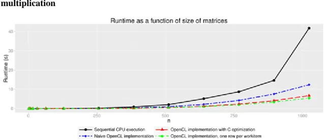
6.1. Comparison of matrix multiplication with the CPU and naive OpenCL implementations ... 129
6.2. Comparison of the CPU and OpenCL implementations of matrix multiplication ... 133
6.3. Comparison of the CPU and OpenCL implementations of matrix multiplication ... 135
6.4. Comparison of the CPU and OpenCL implementations of matrix multiplication ... 136
6.5. Comparison of the CPU and OpenCL implementations of matrix multiplication ... 138
7.1. The representation of digital grayscale images ... 141
7.2. Steps of convolution filtering ... 143
7.3. Some filters and the corresponding filtered images. The identical filter ((a)) results the original image; the Sobel filters are used to emphasize the intensity changes in the x and y directions ((b), (c)); the Gauss- filter with standard deviation 3 decreases the sharpness of the image ((d)) ... 144
7.4. The "Lena" image and the image filtered by Gaussian filter (σ=16) ... 148
7.5. Comparison of the CPU and OpenCL implementations ... 151
7.6. Comparison of CPU and OpenCL implementations ... 151
7.7. Comparison of CPU and OpenCL implementations. ... 152
7.8. The comparison of CPU and OpenCL implementations ... 157
8.1. The original and the resized Lena image ... 180
9.1. Example histograms ... 188
9.2. The histograms of correctly, under- and overexposed images ... 190
9.3. Under- and overexposed images before and after histogram equalization ... 191
9.4. A CT image and its histogram ... 193
9.5. Comparison of the CPU and OpenCL implementations ... 197
9.6. Comparison of the CPU and OpenCL implementations ... 198
9.7. Comparison of the CPU and OpenCL implementations ... 200
9.8. Comparison of the CPU and OpenCL implementations. ... 203
9.9. Comparison of the CPU and OpenCL implementations ... 207
10.1. The graph of the square wave function ... 211
10.2. The first elements of the series defined by equation 10.3, where e1, e2, ... denote terms of the summation ... 211
10.3. The wave functions synthesizing the real part of the complex vector x. ... 216
10.4. The wave functions synthesizing the imaginary part of the complex vector x. ... 218
10.5. The comparison of CPU and OpenCL implementations ... 225
10.6. The comparison of CPU and OpenCL implementations. ... 227
10.7. The comparison of CPU and OpenCL implementations ... 229
10.8. The comparison of CPU and OpenCL implementations ... 231
10.9. The comparison of CPU and OpenCL implementations ... 232
10.10. The indexing scheme of the fast Fourier transform ... 234
10.11. The comparison of CPU and OpenCL implementations. ... 238
10.12. The comparison of CPU and OpenCL implementations ... 243
11.1. Some images of the simulation N= 10 000, steps= 100 and dt= 0.001 ... 253
11.2. Comparison of the sequential CPU and naive OpenCL implementations ... 258
11.3. Comparison of the CPU and OpenCL implementations ... 259
11.4. Comparison of the CPU and OpenCL implementations ... 260
11.5. Comparison of the CPU and OpenCL implementations. ... 261
11.6. Comparison of the CPU and OpenCL implementations ... 262
11.7. Comparison of the CPU and OpenCL implementations ... 263
12.1. Two screenshots of the application ... 274
14.1. Online search trends for OpenCL and CUDA in California ... 288
B.1. The test graph ... 301
C.1. The input and output of the application demonstrating the use of function readPGM and writePGM 307 C.2. The input and output of the application demonstrating the use of PNG I/O functions ... 312
List of Tables
1.1. Comparison of Intel Pentium 4 (2001), Intel Q6600 (2006) and Intel i7-3970X (2013) (The processing units of GeForce 256 are not general purpose processors, they are implementing only the graphics
pipeline. Accordingly, its possible applications are highly limited.) ... 2
1.2. Comparison of NVidia GeForce 256 (2001), NVidia 8600 GTS (2006) and NVidia 690 GTX (2012) 3 4.1. The constants specifing the platform properties, the types and descriptions of properties that can be get using the function clGetPlatformInfo ... 30
4.2. The constants specifing the types of devices that can be queried by the function clGetDeviceIDs 32 4.3. The constants specifying the properties that can be queried by function clGetDeviceInfo and the types and descriptions of the properties ... 33
4.4. The constants defining the properties of partitioning, the types and descriptions of the properties 40 4.5. The constants, specifying the properties related to subdevices, the types and descriptions of the properties ... 40
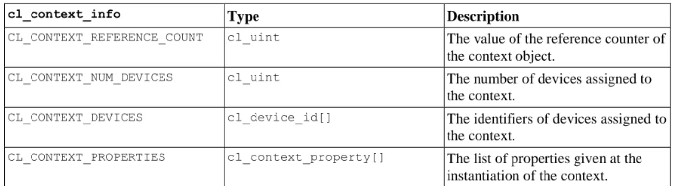
4.6. The constants specifying the properties, the types and descriptions of properties that can be queried by function clGetContextInfo ... 43
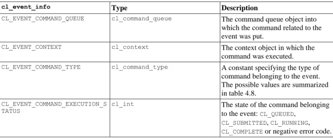
4.7. The constants specifying the properties, the types and descriptions of properties, that can be queried by the clGetEventInfo function ... 48
4.8. The constants specifying commands that can be put into a command queue ... 48
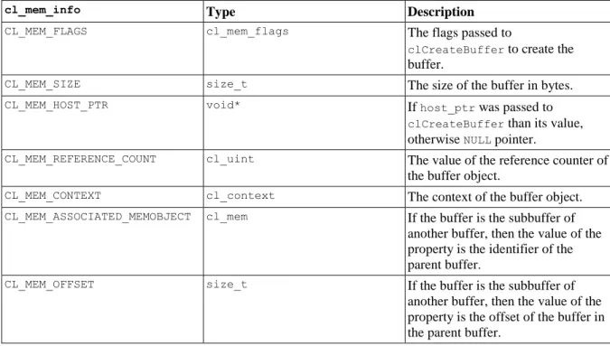
4.9. The constants defining the possible properties of buffer objects and a short description of the properties ... 50
4.10. The constants specifying the properties of buffer objects and the types and short descriptions of the properties. ... 62
4.11. The most important options of the compilation process ... 69
4.12. The most important options of the linking process ... 70
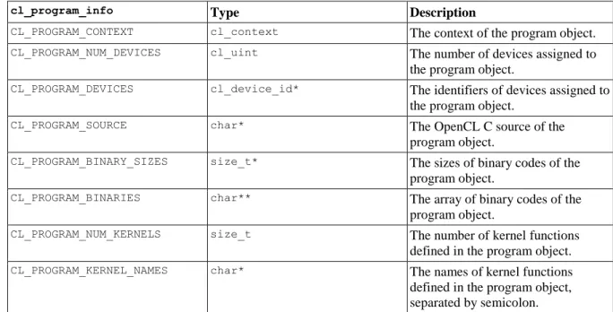
4.13. The constants specifying the properties program objects, their types and descriptions ... 73
4.14. The constants specifying the properties of the build process, their types and descriptions .... 73
4.15. The constants specifying the properties of kernel objects and the types and short descriptions of the properties ... 86
4.16. The constants specifying the properties of kernel arguments, the types and short descriptions of the properties ... 87
8.1. The possible values of the field cl_channel_order ... 161
8.2. The possible values of cl_channel_order and their short descriptions. ... 163
8.3. The fields of structure image_descriptor ... 164
8.4. The possible image object types ... 165
8.5. The constants specifying the properties, the types and short descriptions of the properties that can be queried by the function clGetImageInfo ... 170
8.6. The constants specifying the properties, the types and descriptions of the properties that can be queried by the function clGetSamplerInfo ... 172
A.1. The most important macros of cmake ... 294
A.2. The most important built-in variables of cmake ... 295
List of Examples
2.1. helloWorld.k ... 11
2.2. helloWorld.c ... 12
4.1. error.h ... 26
4.2. error.c ... 26
4.3. platform.c ... 30
4.4. device.c ... 35
4.5. context.c ... 43
4.6. memory.c ... 55
4.7. memory.c: 53-69 ... 56
4.8. memory.c: 55-82 ... 57
4.9. memory.c: 49-92 ... 59
4.10. memory.c: 53-58 ... 60
4.11. memory.c: 53-58 ... 61
4.12. memory.c: 55-68 ... 63
4.13. memory.c:52-70 ... 64
4.14. memory.c:55-70 ... 65
4.15. kernelio.h ... 75
4.16. kernelio.c ... 75
4.17. secondOrder.k ... 76
4.18. build.c ... 76
4.19. secondOrder.k ... 79
4.20. discriminant.k ... 80
4.21. secondOrder.k ... 80
4.22. build.c:45-59 ... 80
4.23. discriminant.k ... 80
4.24. secondOrder.k ... 80
4.25. build.c:45-65 ... 81
4.26. discriminant.k ... 81
4.27. discriminant.k ... 81
4.28. secondOrder.k ... 81
4.29. compilelink.c ... 81
4.30. kernel.c ... 88
4.31. sqrtKernel.k ... 91
4.32. ndrange.c ... 92
4.33. printKernel.k ... 94
4.34. task.c: 64-104 ... 94
4.35. nativeKernel.c ... 96
5.1. vectorTypes1.k:3-6 ... 101
5.2. vectorTypes2.k:3-14 ... 101
5.3. vectorTypes3.k:3-11 ... 101
5.4. vectorTypes4.k:3-17 ... 102
5.5. vectorTypes5.k:3-13 ... 102
5.6. vectorTypes6.k:3-17 ... 103
5.7. vectorTypes6.k:3-4 ... 103
5.8. operators.k:3-11 ... 105
5.9. qualifiers.k ... 106
5.10. primeKernel.k ... 109
5.11. localMaximum.k ... 110
5.12. betaKernel.k ... 112
5.13. commonBits.k ... 113
5.14. loadStore.k ... 114
5.15. localMemory.k ... 115
5.16. localMemory.k ... 117
5.17. count.k ... 119
5.18. count.k ... 119
5.19. printf.k ... 120
6.1. stopper.h ... 123
6.2. stopper.c ... 124
6.3. matmul.c ... 125
6.4. CMakeLists.txt ... 125
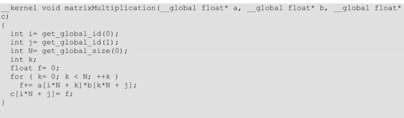
6.5. matrixMultiplication.k ... 126
6.6. matrixMultiplication.k ... 127
6.7. openclinit.h ... 130
6.8. openclinit.c ... 130
6.9. openclinit.c ... 131
6.10. matrixMultiplication.k ... 133
6.11. matrixMultiplication.k ... 134
6.12. matmul.c:108 ... 134
6.13. matrixMultiplication.k ... 135
6.14. matrixMultiplication.k:4 ... 136
6.15. matmul.c:89-91 ... 136
6.16. matrixMultiplication.k ... 137
6.17. matmul.c:46-51 ... 137
6.18. matmul.c:115 ... 138
7.1. filter.h ... 146
7.2. filter.c ... 146
7.3. app.c ... 147
7.4. filter.k ... 149
7.5. app.c ... 149
7.6. filter.k ... 151
7.7. filter.k ... 152
7.8. filter.k ... 153
7.9. filter.k ... 155
7.10. filter.k ... 155
7.11. filter.k ... 155
8.1. image.c ... 168
8.2. resampleKernel.k ... 177
8.3. resize.c ... 178
8.4. image.c ... 183
8.5. resize.c ... 184
9.1. histogram.c ... 194
9.2. histogram.k ... 195
9.3. histogram.c ... 195
9.4. histogram.k ... 197
9.5. histogram.k ... 198
9.6. histogram.k ... 199
9.7. histogram.k ... 201
9.8. histogram.k ... 203
9.9. histogram.c ... 205
10.1. dft.c ... 221
10.2. dft.k ... 223
10.3. dft.c ... 223
10.4. dft.k ... 226
10.5. dftKernel.k ... 227
10.6. dftKernel.k:91-103 ... 228
10.7. dftKernel.k:12-18 ... 229
10.8. dftKernel.k:64-65 ... 229
10.9. dftKernel.k ... 230
10.10. dftKernel.k ... 231
10.11. dftKernel.k:0-26 ... 234
10.12. dftKernel.k:27-52 ... 235
10.13. fft.c ... 235
10.14. dftKernel.k ... 239
10.15. fft.c ... 240
11.1. simulate.c:72-112 ... 251
11.2. simulate.c:9-19 ... 251
11.3. simulate.c:21-53 ... 251
11.4. simulate.c:55-71 ... 252
11.5. simulate.k ... 255
11.6. platform.c:25:166 ... 256
11.7. simulate.k ... 259
11.8. simulate.k ... 260
11.9. simulate.k:1-1 ... 261
11.10. simulate.k ... 261
11.11. simulate.k ... 262
12.1. CMakeLists.txt ... 269
12.2. gravity.c:1-27 ... 269
12.3. gravity.c:28-161 ... 270
12.4. gravity.c:162-245 ... 272
12.5. gravity.c:246-256 ... 273
12.6. gravity.c:274-284 ... 275
12.7. gravity.c:252-272 ... 275
12.8. gravity.c:181-213 ... 276
12.9. gravity.c:71-163 ... 276
12.10. gravity.c:29-53 ... 278
13.1. vectorAdd.k ... 283
13.2. vectorAdd.cu ... 283
13.3. hostOpenCL.c ... 283
13.4. hostCUDA.c ... 284
13.5. webcl.html ... 285
A.1. dlib/dlib.h ... 291
A.2. dlib/dlib.c ... 292
A.3. slib/slib.h ... 292
A.4. slib/slib.c ... 292
A.5. app/main.c ... 292
A.6. CMakeLists.txt ... 293
A.7. slib/CMakeLists.txt ... 293
A.8. dlib/CMakeLists.txt ... 293
A.9. app/main.c ... 293
A.10. CMakeLists.txt ... 296
A.11. FindOpenCL.cmake ... 296
A.12. CMakeLists.txt ... 298
B.1. results-seq.dat ... 300
B.2. results-par.dat ... 300
B.3. figure.R ... 301
C.1. pgmio.h ... 305
C.2. pgmio.c ... 305
C.3. image.c ... 307
C.4. pngio.h ... 309
C.5. pngio.c ... 309
C.6. image.c ... 311
C.7. image.c ... 312
Chapter 1. Introduction
1. The history of OpenCL
Parallel programming technologies are present in the practice of programming since the late 1970s. However, the popular x86 architecture contained only one CPU enabling only functional parallelism1 until the middle of the 2000s. Data parallelism2 was not available to solve computationally expensive problems on desktop computers in parallel. Although desktop computers could be organized into clusters, the computers could communicate on the network and work on subproblems of computationally expensive problems in synchronized ways, the hardware contained only one CPU. Thus, it was an extremely expensive investment to create the circumstances of data parallel distributed computing, available only for the largest computing centres.
Until the beginning of 2000s, the keywords of processor developments were decreasing of the size of transistors and increasing of frequency of CPU clock. When the frequency reached the limen of about 3 GHz, physical limitations appeared: the energy dissipated in the wires of the processor is proportional with the square of the clock frequency. When the frequency is kept around 3 GHz, the cooling of the hardware is still feasible and the electric power is acceptable, however, at higher frequencies the operation becomes too expensive. Thus, the developments have taken another direction: the clock frequency was kept in the range 1-3 GHz and the inner structure of the processors was improved along decreasing transistor size. At one point, the size of transistors and also their electric power became small enough to make the first, general purpose, multi-core CPU for desktop computers.
The first multi-core processor was POWER4, released by IBM in 2001. POWER4 was part of the POWER- series of processors and reckon as a very specific device, however, in 2005, the processors AMD Athlon 64 X2 and Intel Pentium D made the technology available for desktop computers, as well. These many-core CPUs could be programmed with the mature technologies worked out for functional parallel programming mostly, like POSIX threads (Pthreads). To increase the efficiency Intel developed its own parallel programming kit, called Intel Threading Building Blocks (TBB), which is similar to Pthreads in the sense that both allow thread based parallelism. In the same time Open MultiProcessing (OpenMP) - allowing parallelization by simple compiler directives - became very popular and supported by the commonly used compilers. Intel have taken up the development of Cilk, and as a competitor of OpenMP, Intel released its own compiler directive based parallel programming technology, called Intel Cilk Plus. Microsoft released C++ AMP for Visual Studio and Windows, and many more parallel programming technologies have been and are developed currently (OpenACC, OpenHMPP) for C and C++. Several technologies of parallel programming were present when the first general purpose many-core processors appeared, and many technologies have been developed since then. To demonstrate the amount and direction of hardware developments the properties of Intel Pentium 4 (2001), Intel Q6600 (2006) and Intel i7-3970X (2013) are compared in table 1.1.
One of the most powerful tension of hardware developments is the computer game industry. The sequels of popular games are released year-by-year, and the basic requirement of the market is to make the games have significantly better graphical visualization than last year. Accordingly, the graphical processing unit (GPU) has to develop year-by-year significantly, as well. This trend can be qualitatively characterized by some screenshots from the sequels of Need for Speed (released by EA Games) covering the last twenty years (see figure 1.1).
Beside the more detailed graphical visualization, it is worth to mention that the size of the screens has increased more than six times, from 640×480 to 1920×1080. Furthermore, the number of displayed colors has also increased from 28=256 to the True Color standard 232=4294967296. Thus, the better visualization requires the use of more detailed models and the solution of more and more expensive rendering problems, as well.
When real-time 3D visualization became generally available, graphics accelerator cards aided the work of graphics cards to enable the real-time mapping of 3D coordinates to 2D. In the middle of the 1990s, the 0th
1We call functional parallelism when the codes running parallel are different, do not use the CPU heavily and usually perform a kind of slow I/O operation. Functional parallel solutions are behind the interactive, graphical user interfaces. For example, when a browser loads a web page, the functions of the window (menu, buttons) are still available, the user does not have to wait to load a page completely to switch to another tab. The browser is doing two operations in the same time: loads the page through a relatively slow I/O connection and listens the actions of the user. Naturally, functional parallelism can be applied with one CPU, as well. Although the number of executed instructions is not increased, the software becomes more user-friendly and the parallel organization of slow operations increases the utilization of the CPU.
2We call data parallelism when the elements of a data set have to be processed by the same code and more than one CPU is executing that code on different parts of the data. With parallel implementation the time used to process the data set can be reduced, since the number of instructions executed in a given time is increased.
generation of graphics cards and accelerator cards (3Dfx Voodoo, NVidia TNT, ATI Rage) were able to compute one pixel at a time, and only some parts of the graphics pipeline3 were implemented in hardware level. The 1st generation of graphics cards (like newer elements of the 3Dfx Voodoo series) could carry out more and more operations related to visualization, and the members of the 2nd generation (NVidia GeForce 256, ATI Radeon 7500 and variants) implemented all steps of the 3D => 2D mapping at the hardware level. The concept of GPU appeared also that time. Besides, NVidia GeForce 256 had four different graphics pipelines, enabling the parallel computation of four pixels, thus, parallelism appeared on graphics cards. Development had not stopped:
members of the 3th generation (NVidia GeForce 3 and ATI Radeon 8500, 2001) allowed the limited programming of the graphics pipelines, that is, the processing of 3D data on the hardware could be programmed through so called shader languages, similar to Assembly. The 4th generation (NVidia GeForce FX, ATI Radeon 9700) improved the parameters of the hardware (amount of memory, clock frequency, etc.) and extended the programmable operations of the pipelines.
Obviously, developers recognized the high computing capacity of graphics cards and tried to utilize their capabilities through the graphical programming kits, like OpenGL and DirectX. The arrays of data were uploaded to the memory of graphics cards as texture, and the shader languages were used to code the processing steps that are not necessarily related to graphics. When the GPU carried out the processing of the data as texture, the results were downloaded as texture and converted to the desired representation. Nevertheless, the GPU was used for general purposes. This approach is referenced in the literature as General Purpose GPU or GPGPU.
With the 5th generation (NVidia GeForce 6 and ATI Radeon X800, 2004) the first high level languages (allowing also conditional statements and loops) appeared for the programming of the graphics pipeline, aiding the general purpose utilization of GPUs. The vendors of graphics cards have recognized the interests for GPGPU, and invested enormous resources into the research and development of the concept and technology. As a result, the first members of 6th generation (NVidia GeForce 8000 series) appeared in 2006, containing straightly general purpose processors, so called Streaming Multiprocessors. Furthermore, a general purpose programming kit, called NVidia Compute Unified Device Architecture (NVidia CUDA) -- containing libraries and applications aiding the programming of NVidia cards -- became also available. In the same time, AMD has also introduced general purpose GPUs and the Stream Computing SDK, which supports their programming.
The next and present-day GPU generations have followed the steps of CPU developments: the frequency of system clock, the amount of memory, the bandwidth of memory access and the number of processors are increased. However, unlike CPUs, GPUs have parallelism from the beginning of the 2000s, and since then the number of parallel pipelines has increased 2-3 orders of magnitude. In table 1.2 some properties of NVidia GeForce 256 (2001), NVidia 8600 GTS (2006) and NVidia 690 GTX (2012) are given. Comparing the properties of CPUs and GPUs from the same years, it is easy to see that contemporary GPUs contain three times as many transistors as contemporary CPUs. Furthermore, the number of parallel computing units is 500 times greater.
Note that the processors of graphics cards are still not so "general" as CPUs. The computing power of GPUs can be utilized only with well parallelizable problems. Considering the inner structure of CPUs, it is up with some years of development, but considering the number and cooperation of computing units, GPUs are a few years before CPUs.
Considering the inner structure of one processor as a hardware element, an obvious convergence can be recognized: the processor tends to become an array of many general purpose processor cores or computing units.
CPUs and GPUs are approaching this structure from different directions: in CPUs the number of general purpose processor cores is increased; in GPUs the generality and individuality of the many computing units is increased. This can be well observed in the Accelerated Processing Unit (APU) developments of AMD. The origins of APU are the Fusion developments of AMD and ATI (later bought up by AMD). The high performance GPU and CPU are not distinct hardware elements any more, both of them are integrated into a single chip, providing faster and symmetric access to system memory, and some peripherals, as well.
Table 1.1. Comparison of Intel Pentium 4 (2001), Intel Q6600 (2006) and Intel i7-3970X (2013) (The processing units of GeForce 256 are not general purpose processors, they are implementing only the graphics pipeline. Accordingly, its possible applications are highly limited.)
3Independently from the field of the application (CAD softwares, games, etc.), the same processing steps have to be carried out to generate a well-looking 2D image from a set of 3D coordinates and polygons. The sequence of these steps is called the graphics pipeline: model and camera transformations, lighting and shading, projection, clipping, rasterization, texturing, displaying.
Name Pentium 4 Q6600 i7-3970X
Number of processor cores 1 4 6 (12)
Frequency 1.3 GHz 2.4 GHz 3.5 GHz
Number of transistors 125 million 582 million 2,27 billion
Size of cache 256 KB 8 MB L2 15 MB L3
Table 1.2. Comparison of NVidia GeForce 256 (2001), NVidia 8600 GTS (2006) and NVidia 690 GTX (2012)
Name GeForce 256 NVidia 8600 GTS NVidia 690 GTX Number of computing
units
0 4 64
Number of processing units
4 32 3072
Memory 32MB 256 MB GDDR3 4096 MB GDDR5
Bandwidth of memory access
3 GB/s 32 GB/s 384 GB/s
Number of transistors 23 million 289 million 7.1 billion
Figure 1.1. Screenshots from the sequels of Need for Speed released by EA Games
Need for Speed II (1997) Need for Speed: Porsche Unleashed (2000)
Need for Speed: Underground (2003) Need for Speed: Carbon (2006)
Need for Speed: Undercover (2008) Need for Speed: Hot Pursuit (2010)
Need for Speed: Most Wanted (2012)
Altogether, in the middle of the 2000s the first many-core processors appeared with many related technologies, and in the same time, the vendors of GPUs have also provided technologies to utilize the computing capacity of them for general purposes. The fast development of the various hardware related technologies made the developers land in difficulty, since the technologies developed to program parallel CPUs were not compatible with GPUs, and vice versa. Moreover, the development kits of the the greatest GPU vendors (NVidia CUDA, ATI Stream Computing) were neither compatible with each other.
Although Apple does not deal with processor production, its unarguable market position allows Apple to pressure hardware vendors heavily. Thus, the next milestone along the way to OpenCL was put down by Apple.
Due to the intervention of Apple, the biggest vendors (ATI, Intel, NVidia, IBM) joined and worked out the first draft of Open Computing Language (OpenCL), which enables the portable and interoperable programming of their high computing power hardware elements. The draft was submitted to Khronos Group4, where the OpenCL Working Group was founded to manage the development of OpenCL. Thanks to the collaboration, the OpenCL 1.0 specification was released in december 2008.
Note that OpenCL is only a specification, a recommended standard for high performance computing. At the time of its appearance, there were no driver implementations supporting it. However, after the release, AMD preferred to support OpenCL instead of its own GPGPU technology, and NVidia also promised the full support of OpenCL 1.0 in its GPU Computing Toolkit. In the middle of 2009 the first OpenCL supporting drivers were released by NVidia and AMD, that is, one year later that the idea of OpenCL appeared, the technology became available for everyone. The quick advances and developments became permanent for the next years: in June, 2010, Khronos Group published OpenCL 1.1 containing many new tools and in November, 2011, the current standard, OpenCL 1.2 was released providing many new features for parallel programming. In June 2013 the draft of OpenCL 2.0 was published on the website of Khronos Group for online and public discussion.
During the developments of OpenCL, beside NVidia and AMD, many hardware vendors joined as supporters, like IBM, Intel and S3. Comparing to other parallel programming toolkits, the significance of OpenCL is that it allows parallel programming in heterogeneous environments and it is supported by the biggest vendors. This is more or less an outstanding example for collaboration, only the DirectX and OpenGL developments have similar support. In OpenCL related topics one can often meet the term GPU, however, it is worth to note, that OpenCL can be used to program GPUs and CPUs, as well. Particularly, modern many-core processors are able to run OpenCL applications if the proper drivers are installed. Moreover, the programs developed to run parallel on GPUs can be executed parallel on CPUs without any modification. Nevertheless, the architecture of GPUs is designed to solve well-parallelizable problems, thus, still much larger computational power can be achieved
4The Khronos Group is a non-profit organization, founded in 2000 by the largest companies (ATI Technologies, Intel Corporation, NVidia, Silicon Graphics, Sun Microsystems, etc.) related to multi-media. The aim of the organization is to manage the developments of the open source standards of multi-media, like OpenGL, WebGL, OpenVG, etc.
when GPUs are used for the execution of OpenCL programs. Accordingly, most of the sample codes presented and discussed in the rest of the book are developed and tested on GPUs to gain the highest performance. The computing power achievable with GPUs can be demonstrated by considering the architecture and organization of the world's leading supercomputer, Cray Titan. The Cray Titan contains 18.688 AMD Opteron 6274 CPUs, each of them having 16 cores, altogether 299.008 CPU cores. Furthermore, Cray Titan also contains 18.688 NVidia Tesla K20X GPUs, each GPU having 2688 CUDA cores, altogether more than 50 million CUDA cores.
In practice, the only task of the CPUs is to control and manage the operations and tasks performed with the GPUs. The problems are solved generally on the GPUs. The computing power of Cray Titan is 17.59 petaFLOPS5, that is, 17.59×10¹⁵ floating point operations can be performed in 1 second. To illustrate how huge this number is, imagine that all the people of the world can perform one simple operation (for example addition) with real numbers in a second. With that computing power, humanity should compute for 29 days continuously to perform as many operations as Cray Titan can do in a second. Comparing Cray Titan to desktop hardware, Pentium 4 CPUs perform about 6 GFLOPS, today's top processor, Intel Core i7 performs about 100 GFLOPS.
The series 600 of NVidia GeForce GPUs can reach about 3 TFLOPS.
2. The present and future of OpenCL
The developments have not stopped: both AMD and Intel released their OpenCL 1.2 implementations in 2012;
Altera released the first FPGA card that can be programmed through OpenCL; the first tests of smartphone drivers supporting OpenCL are ready; and newer and newer programs utilize the capabilities of OpenCL. The advances have got stuck in only one direction: the probable greatest vendor, NVidia seems to stop supporting OpenCL. In May 2013 NVidia still has not implemented OpenCL 1.2. Many news appeared that NVidia stops supporting OpenCL and focuses on its very similar, but hardware dependent6 alternative, the CUDA technology.
In fact, NVidia drivers support only OpenCL 1.1; the release of NVidia drivers supporting 1.2 have not been announced and the OpenCL supporting homepage of NVidia seems to be out-of-date. Developers are protesting, petitions were started to make NVidia continue the support of OpenCL. In the same time, it is also possible that NVidia focuses now on the next versions of CUDA and its future Maxwell- and Volta-architecture graphics cards to strengthen its market position, and returns to OpenCL soon.
All of this is mentioned, because we can not ignore the fact that the largest part of OpenCL supporting devices comes from NVidia. Therefore, throughout the book, when we discuss OpenCL functionalities, we always refer to the version of OpenCL it has appeared with. Thus, indirectly stating whether or not it can be used with NVidia products.
3. OpenCL and Flynn-classes
The main purpose of OpenCL is to make the parallel programming of high performance computing hardware devices uniform. These devices include GPUs, CPUs, FPGA cards7 and other accelerating hardware as well.
The common property of OpenCL supporting hardware devices is that each of them contains many computing units or processor cores. The reason for that is the nature of hardware developments: At the beginning they had different functionalities, but the developments of the hardware faced similar physical constraints (like the frequency of system clock), and the developments started to have similar directions: with the decrease of size of transistors, more and more computing units can be formed.
To put OpenCL technology on the map of already evolved parallel hardware and software solutions, we briefly overview the so-called Flynn-classes covering most of the possible approaches.
• SISD (Single Instruction Single Data Stream) - There is no parallel execution, only one data element is processed at a time, and all data is processed sequentially with the same instructions. According to their architecture, the conventional, one-CPU desktop computers implement the SISD approach. Although time-
5FLOPS (FLoating-point Operations Per Second) is the commonly used unit of computing power. 1 FLOPS is the computing power of the machine able to perform one floating-point operation in a second.
6CUDA can be used to develop for NVidia GPUs only. Thus, OpenCL is much more general. However, due to its specialization, somewhat faster programs can be developed for NVidia with CUDA than with OpenCL.
7As it comes from its name, FPGA cards are arrays of logical gates programmable on the "field". Thus, this is a kind of hardware enabling the modification of its inner wiring even after it is installed. The use of FPGA cards enable the implementation of specific algorithms at the hardware level without the need of expensive hardware developments. One must use the HDL (hardware definition language) language to specify the organization of logical gates and the FPGA card is able to realize it. Thus, the algorithm described with HDL becomes present in the wirings of the hardware, and no target hardware has to be developed.
sharing operating systems makes the user feel like many programs run "parallel" (browser, word processor, etc.), this parallelism is only an illusion: considering a moment, only one instruction is performed, only one program is running.
• SIMD (Single Instruction Multiple Data Stream) - The same sequence of instructions is executed in several instances processing different elements of the data. By definition, SIMD requires many processors to execute the same program in parallel. It is worth to note that the individual processors can run through different paths in the code. Basically, GPU processors have SIMD architecture, the computing units execute the same program but compute different parts of the image to visualize. The SIMD architecture can be used the most efficiently when data-parallel solutions are required and the processing of the data elements can be done independently.
• MISD (Multiple Instruction Single Data Stream) - There is only one data stream, but each data element is processed with different programs on different processors, in parallel. The implementations of the MISD architecture are very rare, only some special devices and solutions fit to this category. The literature mentions mostly the computers processing the stream of flying data of Space Shuttles with several different programs, in parallel.
• MIMD (Multiple Instruction Multiple Data) - Many processors performs different tasks on different data, in parallel. For example, the many-core desktop computers and supercomputers implement MIMD architecture, but the many-core smartphones can be considered as MIMD devices as well.
Obviously, Flynn-classes are theoretical, in practice, the classes can not be differentiated strictly, moreover, the literature has also some uncertainty with specific processors and solutions. GPUs have basically SIMD architecture: in the beginning only some steps of the graphics pipeline were executed in parallel. By time, the SIMD nature of GPUs has merged with the MIMD approach, since today's GPUs can be programmed to run different programs on the computing units in the same time. Nevertheless, the best performance can be achieved if we keep ourselves to the SIMD approach.
OpenCL technology is independent from the hardware and its architecture, therefore the OpenCL specification refers to an abstract hardware, called OpenCL device. The OpenCL device can be any hardware that supports the semantics of the OpenCL specification through its driver. Later on, we will see that the architecture of the abstract OpenCL device is very similar to the architecture of GPU processors. Since GPUs are classified into the SIMD category, the OpenCL technology fits also to the SIMD class the most.
4. What is OpenCL used for?
In its short lifetime, the possibilities of OpenCL were utilized in many disciplines and areas of computing. In the next paragraphs we overview and highlight some developments to demonstrate the wide range of its applications.
OpenCL is often and successfully applied in digital image processing, where the same operations are to be performed on pixels of images or frames of video streams. For example Adobe PhotoShop CS68 and Corel VideoStudio Pro X69 both use OpenCL to accelerate processing if OpenCL compatible devices are available.
Two examples from the open source libraries: GIMP and the GEGL10 library released by the developers of GIMP use OpenCL acceleration. In the highly related field of computer graphics, the photorealistic and in many times physically correct rendering of 3D images can be highly accelerated by OpenCL (Indigo Renderer11).
In mathematics, the Vienna University of Technology released ViennaCL12, a library containing OpenCL optimized methods for linear algebra. The R Linear Inverse Problem Solver13 package uses OpenCL based acceleration to solve inverse problems of linear algebra. These applications can be utilized in numerous disciplines from nuclear imaging to data mining. The Jacket14 package released by AccelerEyes makes OpenCL based parallelization available in Matlab. Furthermore, Wolfram Mathematica 915 also contains methods running
8http://www.adobe.com/products/photoshop.html
9http://www.corel.com/corel/product/index.jsp?pid=prod4900075
10http://www.gegl.org/
11http://www.indigorenderer.com/
12http://viennacl.sourceforge.net/
13http://www.sgo.fi/~m/pages/rlips.html
14http://www.accelereyes.com/
15http://www.wolfram.com/mathematica/
in parallel if OpenCL devices are available. Since OpenCL appeared in Matlab and Wolfram Mathematica, it is applied by many researchers and engineers without realizing they are using it, in fact.
In physical simulations, in the N-body problem or in molecule dynamics the behaviour of bodies or molecules are driven by the same forces, thus, the same programs are to be run for each instance to compute its acceleration, velocity and position. The simulations are closely related to the solution of finite element models, when the problems are described by complex differential equation systems (like Navier-Stokes differential equations for heat transfer), and the solutions are computed by parallel numerical approximations. Many simulation and finite element problems can be solved by the software Abaqus Finite Element Analysis16 and EDEM17, which also utilize OpenCL.
PostgreSQL18 is the first database management system modifying the data stored in databases by OpenCL. For this purpose, a dedicated language, PgOpenCL was developed.
The Biomanycores19 project is dedicated to support the intensively researched fields of bioinformatics.
Biomanycores also utilizes the computing capacity of available OpenCL devices.
From general solutions we highlight the Berkeley Open Infrastructure for Network Computing20 (BOINC) which enables anybody to contribute to the largest computing problems of humanity. In the BOINC framework the subproblems of a problem are solved by volunteers joined to BOINC by installing a simple desktop application.
Obviously, the BOINC client application enables the utilization of available OpenCL devices. For example, BOINC runs the widely known SETI@home21 project searching for the signals and evidences of intelligent life in the universe; and the evidences of gravitation waves are also researched by a BOINC hosted project, called Einstein@home22. In March 2013, BOINC had an average of 9.2 petaFLOPS computing power, that is more than half of the computing power of Cray Titan. Among many components, the power of BOINC is due to its support for OpenCL.
From the popular, everyday software we highlight VLC media player23 applying stability and noise reduction methods to video streams by OpenCL and WinZip24 accelerating the compression and decompression of data when OpenCL devices are available.
Beside user applications, it is worth to mention that the driver support of OpenCL is also continuously increasing. Altera25 just released its first, general purpose high performance Field-Programmable Gate Array (FPGA) cards programmable through OpenCL, thus, bringing the FPGA devices closer to the mainstream programming, allowing the use of OpenCL beside the Hardware Description Languages (HDL).
The OpenCL specification defines C and C++ interfaces. However, in the last years, several interfaces have been developed to extend its applications: later on we discuss WebCL, the JavaScript interface of OpenCL in details; we also highlight the Aparapi26 project enabling OpenCL programming in Java, the PyOpenCL27 library developed for Python and the Ruby-OpenCL28 package for Ruby.
According to some news appeared in the beginning of 2013, the Nexus 4 smartphone and Nexus 10 tablet PC released by Google have some primary support for OpenCL, that is, one can write programs for Android using the graphics processors of the device through OpenCL.
It can be easily seen that OpenCL is utilized from supercomputers through FPGA cards to smartphones, from the largest scientific problems through Photoshop to everyday programs, like WinZip and VLC Player. Since the use of OpenCL can enable sensible increase in performance, the trend does not seem to stop, moreover, some experts state that OpenCL will really "start up" in 2014. Assumably this may become reality, since OpenCL is already widely spread, despite of that it has appeared the first time only somewhat more than 4 years ago.
16http://www.3ds.com/products/simulia/portfolio/
17http://www.dem-solutions.com/software/edem-software/
18http://www.postgresql.org/
19https://biomanycores.org/
20http://boinc.berkeley.edu/
21http://setiathome.berkeley.edu/
22http://www.einstein-online.info/spotlights/EaH
23http://www.videolan.org/vlc/
24http://www.winzip.com/win/en/index.htm
25http://www.altera.com/
26http://code.google.com/p/aparapi/
27http://mathema.tician.de/software/pyopencl/
28http://ruby-opencl.rubyforge.org/
5. About the book
5.1. The aim and use of the book
The aim of the book is to introduce the reader into the OpenCL technology. The only requirement for the reader is to know the main features of the ANSI C language. Accordingly, we focus on the C interface of the OpenCL technology and we will utilize the ANSI C knowledge in discussion of the OpenCL C language that is used to write the parallel kernels running on the OpenCL device.
In the first chapters the terminology of OpenCL is presented, and the architecture of the abstract OpenCL device, technology and the functions of the OpenCL library are described. The usage of the functions are demonstrated by many sample codes throughout the book. In the second half of the book some complex examples are discussed in detailed case studies. For each case study we briefly describe the mathematical background and aid the navigation of the reader in the field with references to corresponding textbooks. The case studies are important parts of the books, since the OpenCL specification describes only the semantics of the functions, the "tricks" of writing efficient OpenCL programs can be learned by analysing and understanding the philosophy of efficient sample codes.
Readers can test their understanding and also practice OpenCL by solving the exercises at the end of the chapters. These exercises also deepen the knowledge of the reader in the topics of the case studies that are closely related to the industrial and scientific applications of OpenCL.
The difficulty of the exercises is marked by a three-element scale of star (★) symbols. One star (★) indicates easy exercises, two stars (★★) mark the intermediate problems and three marks (★★★) are used to denote exercises requiring more coding or some mathematical hackery. The book contains exercises of 295 stars altogether. If the book is used in education, due to its technological content, the gradation is intended to be based on administered solutions of the exercises:
• To pass the corresponding course on OpenCL, the student should solve exercises from each chapter with the value of three stars per chapter, at least.
• Furthermore, for the grade 2, exercises of the overall value of 30 stars have to be solved. For the grade 3, exercises with 35 stars; for the grade 4, exercises with 40 stars and for the best mark 5, exercises of the overall value of 45 stars have to be solved.
5.2. What is the book based on?
The book is based on several sources of OpenCL related documents and descriptions. All of that is recommended for the reader to deepen his knowledge about the topic. First of all, the official OpenCL 1.129 and OpenCL 1.230 specifications are available at the homepage of the Khronos Group. From the printed literature we highly recommend the books [5], [14], [11], [12] and [16]. Since the specification leaves several details for the implementations and the implementations sometimes extend OpenCL, it is highly advised to go through the descriptions of the available hardware environments: AMD31, Intel32. Further, useful and actual informations can be found in the forum topics related to OpenCL and one can also learn a lot by going through and understanding the codes written by experts: AMD33, Intel34, NVidia35.
5.3. Hardware environment
The run tests are performed on two OpenCL devices. The sample codes using the new functions of OpenCL 1.2 are executed with the AMD APP implementation of OpenCL on CPU and the codes using OpenCL 1.1 only are tested with the NVidia implementation of OpenCL using the device 8600 GTS GPU.
29http://www.khronos.org/registry/cl/specs/opencl-1.1.pdf
30http://www.khronos.org/registry/cl/specs/opencl-1.2.pdf
31http://www.siliconwolves.net/frames/why_buy/AMD_Accelerated_Parallel_Processing_OpenCL_Programming_Guide.pdf
32http://software.intel.com/sites/default/files/m/e/7/0/3/1/33857-Intel_28R_29_OpenCL_SDK_User_Guide.pdf
33http://developer.amd.com/tools-and-sdks/heterogeneous-computing/amd-accelerated-parallel-processing-app-sdk/samples-demos/
34http://software.intel.com/en-us/articles/intel-sdk-for-opencl-applications-xe-samples-getting-started
35https://developer.nvidia.com/opencl
Chapter 2. My first OpenCL program
This chapter is twofold. On the first hand we set up the software environment for using OpenCL, on the other hand while testing the environment we implement the first OpenCL program and roughly discuss the main parts of it, as well as the steps of compilation and linking. After this chapter the reader will have a preliminary view about the structure of OpenCL programs, and they can be sure that their own software and hardware environment is suitable and properly configured for OpenCL programming. In the same time we shortly discuss some use cases of the source code managing cmake toolkit.
1. Programming environment
In general, high performance computing is carried out in Linux based operating systems. The author works on the Debian based Kubuntu 13.04 system and all the sample codes presented, and discussed in the rest of the book are run and tested in this environment. To try and test the sample codes in the book we also propose the use of some kind of Linux distribution. Note that OpenCL codes are highly portable, namely, one can run the codes on Windows or Apple systems without any modification, but the development and testing is much simpler on Linux due to its fine scripting mechanisms.
The syntax of OpenCL is specified in header files. However, just like many other open source standards, the specification and implementation are separated from each other. All the vendors supporting OpenCL must make their own implementation of the OpenCL standard fitting their devices. The header files can be purchased in several ways. On the one hand, they can be downloaded from the webpage1 of the Khronos Group, on the other hand, several Linux distribution has a package in its repository, dedicated for the OpenCL headers. For example, in the case of Ubuntu distributions, one can simply get the header files by installing the package opencl- headers.
root@linux> apt-get install opencl-headers
After the installation of the package, let's check out wether the files are available in the default /usr/include/CL directory:
user@linux> ls -l /usr/include/CL/
total 1060
-rw-r--r-- 1 root root 4859 Nov 15 2011 cl_d3d10.h -rw-r--r-- 1 root root 4853 Apr 18 2012 cl_d3d11.h
-rw-r--r-- 1 root root 5157 Apr 18 2012 cl_dx9_media_sharing.h -rw-r--r-- 1 root root 9951 Nov 15 2011 cl_ext.h
-rw-r--r-- 1 root root 2630 Nov 16 2011 cl_gl_ext.h -rw-r--r-- 1 root root 7429 Nov 15 2011 cl_gl.h -rw-r--r-- 1 root root 62888 Nov 16 2011 cl.h -rw-r--r-- 1 root root 915453 Feb 3 2012 cl.hpp
-rw-r--r-- 1 root root 38164 Nov 16 2011 cl_platform.h -rw-r--r-- 1 root root 1754 Nov 15 2011 opencl.h
Note that the organization of the GL directory containing OpenGL header files is similar to that of the CL headers.
Generally, the OpenCL implementation is available through dynamically linkable program libraries, called shared object (.so) on Linux systems and dynamic-link library (.dll) on Windows. These libraries are usually part of the driver provided for the OpenCL supporting device or available to download on the webpage of the vendor. The writers use NVidia graphics card as OpenCL supporting divice, and accordingly the driver available at the NVidia webpage2 contains the OpenCL implementation itself. After the installation of the driver, the libraries are available at the default /usr/lib directory.
user@linux> ls -l /usr/lib/libOpenCL*
lrwxrwxrwx 1 root root 14 Feb 3 18:03 /usr/lib/libOpenCL.so -> libOpenCL.so.1 lrwxrwxrwx 1 root root 16 Feb 3 18:03 /usr/lib/libOpenCL.so.1 -> libOpenCL.so.1.0 lrwxrwxrwx 1 root root 18 Feb 3 18:03 /usr/lib/libOpenCL.so.1.0 ->
libOpenCL.so.1.0.0
-rwxr-xr-x 1 root root 21296 Feb 3 18:03 /usr/lib/libOpenCL.so.1.0.0
1http://www.khronos.org/registry/cl/
2http://www.nvidia.com/Download/index.aspx?lang=en-us
Once the driver of the OpenCL supporting device is properly installed, the libraries and the header files are available, we are ready to write the first program using the features of OpenCL.
2. Hello world
The aim of OpenCL is to generalize the programming of high performance computing devices by hiding the differences of the hardware itself. As a drawback of generality, the inicialization of the OpenCL environment requires several steps to be done in every program using OpenCL. Therefore, the simplest "Hello world!"
application is much longer than the introductionary programs of other parallel programming technologies, like OpenMP or Pthreads.
The OpenCL can not be discussed in details before the reader get to know the abstract architecture of the OpenCL device. Therefore, one has to get to know many concepts before all the lines of a sample program are clarified. To make the reader have a first impression about these concepts, the structure of OpenCL programs and to have an application that can be used to test if the environment is properly configured, we present a short sample code, discuss its structure and the main steps of the compilation and linking. The sample code simply writes the string "Hello world!" to the standard output, however, the letters of the string are put together on the OpenCL device parallel.
The first step is to write the chunk of code running on the OpenCL device, called the kernel-code. This code is stored in a file having the extension .k, referring to "kernel". In fact, one can use any extension, since this file is not to be compiled neither linked, no compiler or linker should recognize its extension, therefore, we do not have to be strict to any naming convention. The kernel is written in the OpenCL C language, which is an extension of the ANSI C language by adding some elements related to the parallel execution. The OpenCL C language is covered in a later chapter of the book. Anyway, the code can be easily interpreted without knowing the novel elements of OpenCL C.
Example 2.1. helloWorld.k
__kernel void helloWorld(__global char* output) {
int p= get_global_id(0);
switch( p ) {
case 0:
output[p]= 'H';
break;
case 1:
output[p]= 'e';
break;
case 2:
case 3:
case 9:
output[p]= 'l';
break;
case 4:
case 7:
output[p]= 'o';
break;
case 5:
output[p]= ' ';
break;
case 6:
output[p]= 'w';
break;
case 8:
output[p]= 'r';
break;
case 10:
output[p]= 'd';
break;
case 11:
output[p]= '!';
break;
default:
output[p]= '\0';
break;
} }
The parameter of the kernel-function is a string. The kernel determines the index of the kernel instance running parallel and sets the character at the same index of the string to the proper letter. The index of the kernel function, namely, the return value of the function get_global_id is discussed in details later.
The OpenCL functions called from the main function and the main parts of the program are discussed after the source code.
Example 2.2. helloWorld.c
#include <stdio.h>
#include <stdlib.h>
#include <string.h>
#include <CL/opencl.h>
#define ARRAY_SIZE 40
#define MAX_DEVICES 2
#define MAX_PLATFORMS 2
#define MAX_SOURCE_LENGTH 2000
#define ERROR(err, prefix) if ( err != CL_SUCCESS ) printErrorString(stderr, err, prefix);
int printErrorString(FILE* o, int err, const char* p) {
switch(err) {
case CL_SUCCESS: fprintf(o, "%s: Success.\n", p); break;
case CL_DEVICE_NOT_FOUND: fprintf(o, "%s: Device not found.\n", p); break;
case CL_DEVICE_NOT_AVAILABLE: fprintf(o, "%s: Device not available.\n", p); break;
case CL_COMPILER_NOT_AVAILABLE: fprintf(o, "%s: Compiler not available.\n", p);
break;
case CL_MEM_OBJECT_ALLOCATION_FAILURE: fprintf(o, "%s: Mem. obj. app. fail.\n", p);
break;
case CL_OUT_OF_RESOURCES: fprintf(o, "%s: Out of resources.\n", p); break;
case CL_OUT_OF_HOST_MEMORY: fprintf(o, "%s: Out of host memory.\n", p); break;
case CL_BUILD_PROGRAM_FAILURE: fprintf(o, "%s: Program build failure.\n", p); break;
case CL_INVALID_VALUE: fprintf(o, "%s: Invalid value.\n", p); break;
case CL_INVALID_DEVICE_TYPE: fprintf(o, "%s: Invalid device type.\n", p); break;
case CL_INVALID_PLATFORM: fprintf(o, "%s: Invalid platform.\n", p); break;
case CL_INVALID_DEVICE: fprintf(o, "%s: Invalid device.\n", p); break;
case CL_INVALID_CONTEXT: fprintf(o, "%s: Invalid context.\n", p); break;
case CL_INVALID_QUEUE_PROPERTIES: fprintf(o, "%s: Invalid queue properties.\n", p);
break;
case CL_INVALID_COMMAND_QUEUE: fprintf(o, "%s: Invalid command queue.\n", p); break;
case CL_INVALID_HOST_PTR: fprintf(o, "%s: Invalid host pointer.\n", p); break;
case CL_INVALID_MEM_OBJECT: fprintf(o, "%s: Invalid memory object.\n", p); break;
case CL_INVALID_BINARY: fprintf(o, "%s: Invalid binary.\n", p); break;
case CL_INVALID_BUILD_OPTIONS: fprintf(o, "%s: Invalid build options.\n", p); break;
case CL_INVALID_PROGRAM: fprintf(o, "%s: Invalid program.\n", p); break;
case CL_INVALID_PROGRAM_EXECUTABLE: fprintf(o, "%s: Invalid program exec.\n", p);
break;
case CL_INVALID_KERNEL_NAME: fprintf(o, "%s: Invalid kernel name.\n", p); break;
case CL_INVALID_KERNEL_DEFINITION: fprintf(o, "%s: Invalid kernel def.\n", p);
break;
case CL_INVALID_KERNEL: fprintf(o, "%s: Invalid kernel.\n", p); break;
case CL_INVALID_ARG_INDEX: fprintf(o, "%s: Invalid argument index.\n", p); break;
case CL_INVALID_ARG_VALUE: fprintf(o, "%s: Invalid argument value.\n", p); break;
case CL_INVALID_ARG_SIZE: fprintf(o, "%s: Invalid argument size.\n", p); break;
case CL_INVALID_KERNEL_ARGS: fprintf(o, "%s: Invalid kernel arguments.\n", p);
break;
case CL_INVALID_WORK_DIMENSION: fprintf(o, "%s: Invalid work dimension.\n", p);
break;
case CL_INVALID_WORK_GROUP_SIZE: fprintf(o, "%s: Invalid work group size.\n", p);
break;
case CL_INVALID_WORK_ITEM_SIZE: fprintf(o, "%s: Invalid work item size.\n", p);