Research Article
The Impact of Façade Orientation and Woody Vegetation on Summertime Heat Stress Patterns in a Central European Square:
Comparison of Radiation Measurements and Simulations
Noémi Kántor,
1Csilla Viktória Gál,
2Ágnes Gulyás,
1and János Unger
11Department of Climatology and Landscape Ecology, University of Szeged, Egyetem u. 2, 6722 Szeged, Hungary
2School of Technology and Business Studies, Dalarna University, 79188 Falun, Sweden
Correspondence should be addressed to J´anos Unger; unger@geo.u-szeged.hu Received 11 September 2017; Accepted 12 November 2017; Published 15 January 2018
Academic Editor: Hiroshi Tanaka
Copyright © 2018 No´emi K´antor et al. This is an open access article distributed under the Creative Commons Attribution License, which permits unrestricted use, distribution, and reproduction in any medium, provided the original work is properly cited.
Increasing summertime air temperature deteriorates human health especially in cities where the warming tendency is exacerbated by urban heat island. Human-biometeorological studies shed light on the primary role of radiation conditions in the development of summertime heat stress. However, only a limited number of field investigations have been conducted up to now. Based on a 26- hour long complex radiation measurement, this study presents the evolved differences within a medium-sized rectangular square in Szeged, Hungary. Besides assessing the impact of woody vegetation and fac¸ade orientation on the radiation heat load, different modeling software programs (ENVI-met, SOLWEIG, and RayMan) are evaluated in reproducing mean radiant temperature (𝑇mrt).
Although daytime𝑇mrtcan reach an extreme level at exposed locations (65–75∘C), mature shade trees can reduce it to 30–35∘C.
Nevertheless, shading from buildings adjacent to sidewalks plays also an important role in mitigating pedestrian heat stress.
Sidewalks facing SE, S, and SW do not benefit from the shading effect of buildings; therefore, shading them by trees or artificial shading devices is of high importance. The measurement–model comparison revealed smaller or larger discrepancies that raise awareness of the careful adaptation of any modeling software and of the relevance of fine-resolution field measurements.
1. Introduction
Regional climate change is expected to bring rising air temperature values and to increase the frequency, length, and severity of heat waves in Central Europe, and thus in Hungary too [1, 2]. Combined with the peculiar climate of cities, characterized by increased air temperature and reduced ventilation due to the great amount of artificial materials, low vegetation rate, and the complex surface morphology [3], extreme heat events are expected to have more serious impacts on urban environments [4]. Without adaptation to heat waves people shall face deteriorating thermal comfort conditions, which in turn lead to declining working efficiency [5]. Moreover, intensification of heat stress is expected to increase the mortality rates, especially among the vulnerable groups, like infants, elderly people, and those with cardiovascular diseases [6]. In this respect it is worth emphasizing that, among the continents, Europe has the
greatest percentage (24%) of its population aging 60 or over [7]. Furthermore, 73% of the European population already lives in urban areas, and by 2050 this proportion is expected to rise over 80% [7]. In the light of the mentioned warming, aging, and urbanization tendencies, mitigating the impact of extreme heat events should be one of the most important issues in urban planning [8–10].
Researchers in the field of urban human-biometeorology demonstrated that radiation heat load, quantified usually as mean radiant temperature (𝑇mrt) [[11–13] and see Section 2.2], is the main factor of daytime heat stress in summer in midlatitudes, and therefore shading, that is, the reduction of𝑇mrt is the most effective mean of heat stress mitigation in outdoor urban spaces [14–18]. Field measurements and simulation studies conducted at various climate zones (conti- nental, arid, and tropical) have shown that larger tree canopy coverage and higher street aspect ratio (that is, shading by buildings) are generally the most effective design strategies
Volume 2018, Article ID 2650642, 15 pages https://doi.org/10.1155/2018/2650642
against urban heat stress [19–27]. Studies from cities with temperate climates commonly found that shading delivers the greatest human-biometeorological improvement [28–
34]. It must be emphasized that only a limited number of field experiments have been conducted relying on the most accurate six-directional radiation measurement technique up to now, because this technique requires expensive and heavy instrumentation [[11–13] and see Section 2.2].
Numerical models are popular and easily obtainable alternatives of the time- and resource-consuming onsite investigations to determine𝑇mrt. For this purpose commonly used simulation software programs are ENVI-met [35–39], RayMan Pro [40–42], and SOLWEIG [43–46]. Although the number of simulation studies expands rapidly, only few of the modeled results have been validated with accurate onsite measurement. Except [47] that investigated several techniques in their capabilities to obtain𝑇mrt, the available validation studies focused usually only on one of the men- tioned models, although comparison of their performance among different conditions, revealing their benefits and shortcomings, would be of great interest for professional urban planners and landscape designers. Experimental𝑇mrt values were used to validate ENVI-met in Freiburg, Germany [30, 37, 38], while the performance of RayMan was tested in various cities, that is, in G¨oteborg, Sweden [12], in Freiburg, Germany [40–42], in Glasgow, UK [48], and even in Huwei, Taiwan [22, 49]. The latter three validation studies relied on field surveys utilizing globe thermometers, although this technique has been demonstrated to be inappropriate in outdoor conditions [50]. In contrast, there are other studies where the model-measurement comparisons were based on the most accurate six-directional radiation measurement technique (e.g., [12, 30, 37, 38, 42, 47]). The low number of such validation studies can be explained by the expensive sensors, and the time and human-resource intensive nature of these measurements.
According to the above mentioned, this study intends to contribute to the urban human-biometeorological knowl- edge by conducting a detailed analysis of the evolved radia- tion conditions (radiation flux densities from six main direc- tions) and the resulted𝑇mrt differences within a medium- sized rectangular square in Szeged, one of the warmest cities of Hungary. Special emphasis is put on the importance of sidewalks’ exposure to direct irradiation, that is, the fac¸ade orientation of the buildings bordering the square and the role of woody vegetation in mitigating heat stress. Beside assessing the impact of shade trees and different fac¸ade orientations on the radiation heat load in a complex urban setting, this study aims to evaluate and compare ENVI-met, SOLWEIG, and RayMan in their ability to reproduce𝑇mrt.
2. Materials and Methods
2.1. Study Area. The field measurements were conducted in the city of Szeged (46.3∘N, 20.1∘E), the southeastern regional center of Hungary with an urbanized area of 40 km2 [51].
Szeged offers an ideal study environment for urban climate and human-biometeorological investigations as it is built on a flat terrain with slight topographical differences (78–85 m
above sea level), which enables the generalization of the obtained results, (see, e.g., [18, 52]). Urban land use patterns vary across the town, ranging from dense inner-city areas to sparse suburban landscapes, which allow for the development of several local climate zone types [53]. Szeged has a warm temperate climate with rather uniform annual distribution of precipitation. Based on the 1971–2000 climate normal data of Szeged, the yearly amount of precipitation is low (489 mm), while the number of sunshine hours is high (1978 h). The annual mean air temperature is 10.6∘C, and July and August are the hottest months, while January is the coldest [54].
Being one of the warmest cities in Hungary, the urban climate of Szeged is expected to be affected intensively by the warming projected for the Carpathian Basin [55]. Moreover, Szeged is the third most populated city in the country with more than 162,000 permanent residents. These attributes make the city an appropriate place for urban climate and human-biometeorological investigations.
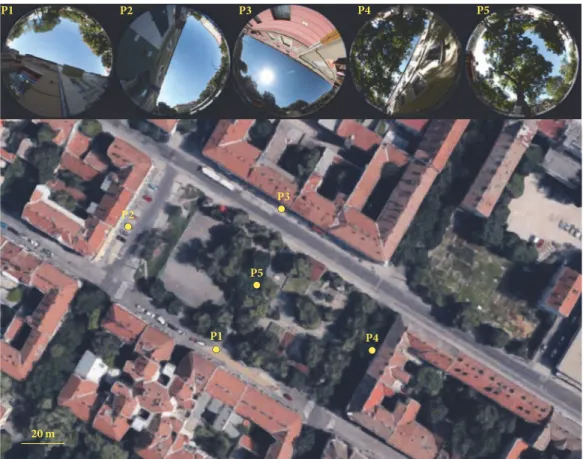
The medium-sized rectangular Bart´ok Square (Figure 1;
core area: 110 m× 55 m, plus the surrounding streets) was selected as the study area for the field measurements and for the assessment of small-scale radiation models. The square is located within a “compact midrise” local climate zone (LCZ 2) in the inner-city [51]. It is an important hub of public transit and pedestrians traffic with two bus stops at its opposite sides. The square offers opportunities for recreation and socialization: there is an asphalt-covered basketball–football court on the WNW part, several small kiosks on the NNE side, and benches located across the place. Thus, the place serves the needs of people of all ages. The well-vegetated central and ESE parts of the square are characterized by 10–20 m tall deciduous trees (e.g.,Platanus×acerifolia, Tilia cordata, Ulmus procera, Sophora japonica, Fraxinus excelsior, andCeltis occidentalis). Beside the shade from trees, parts of the square also benefit from the shading of the adjacent 3-4- story buildings.
Five measurement sites were selected to investigate the radiation load on pedestrians that either walk on the side- walks surrounding the square or linger under the mature shade trees in the central area (Figure 2):
(i) P1, P2, P3, and P4 are located near to buildings encir- cling the square. The nearest fac¸ades to these points are located at SSW, WNW, NNE, and ESE sides, respectively, at ca. 1.3 m distance.
(ii) P5 is in the middle of the square, under a 10-meter tallSophora japonicatree with an app. 13-meter wide crown; the station was placed 2 m north from the trunk of the tree.
2.2. Field Measurements. Two human-biometeorological sta- tions were used to record one-minute averages of all atmo- spheric parameters influencing human thermal comfort (Figure 3). One of the stations was continuously moved around the four lateral measurement points (P1–P4) at 15- minute intervals, while the other remained under the large tree at point P5 during the entire measurement period. Both stations were equipped with a Vaisala WXT 520 weather transmitter to record air temperature (𝑇𝑎), relative humidity,
0 50 100 200 300 400 Meters Bartók Square
Tree height (m) High: 13 Low: 5
High: 119 Low: 80 Builiding height (m) (above ground level)
(above sea level)
N
Figure 1: Bart´ok Square of Szeged, illustrated by an aerial image, site photos, and an object elevation map.
and wind speed. They were also equipped with a rotatable Kipp & Zonen net radiometer to monitor the 3D radiant environment—that is, to record shortwave and longwave radiation flux densities from six perpendicular directions (𝐾𝑖 and 𝐿𝑖 [Wm−2], 𝑖: up, down, east, west, south, and north). By means of telescopic tripods, the sensors were set at 1.1–1.2 m above ground level—at an elevation recommended for human-biometeorological investigations [10].
Typically, in the first position, the arm of the net radiome- ters pointed to the south, while the sensors were faced upwards and downwards. This means that in this position, the two pyranometers and two pyrgeometers measured 𝐾𝑖 and𝐿𝑖separately from the upper and lower hemisphere (𝐾𝑢, 𝐾𝑑,𝐿𝑢,𝐿𝑑). After three minutes, the net radiometers were rotated manually to the second position where the sensors faced east and west (𝐾𝑒,𝐾𝑤,𝐿𝑒,𝐿𝑤). After another 3-minute measurement, the arms were turned 90∘ to measure the radiation flux densities coming from the south and north (𝐾𝑠, 𝐾𝑛,𝐿𝑠,𝐿𝑛). Considering our 26-hour measurement period, this procedure required hundreds of rotations. Taking into account the response time of the sensors, as well as the time delays due to rotation, the first𝐾𝑖and𝐿𝑖records following a rotation were removed. Additionally, to record conditions representative of a new thermal environment, the first three- minute data following relocations were also omitted.
Mean radiant temperature (𝑇mrt[∘C]), a parameter with primary importance in the field of human-biometeorology,
combines all longwave and shortwave radiant flux densities into a single value in ∘C. 𝑇mrt is defined as the uniform temperature of an imaginary black body-radiating surround- ing, which causes the same radiant heat exchange for the human body inside this hypothetical environment as the real, complex 3D radiant environment [11, 13]. In the case of this study,𝑇mrtwas determined based on six𝐾𝑖 and six𝐿𝑖flux densities obtained from three consecutive positions of the net radiometer.
𝑇mrt=√ 𝐾4 ∗+ 𝐿∗
𝑎𝑙× 𝜎 − 273.15 (1) 𝐾∗ = ∑ 𝐾𝑖∗= ∑ 𝑊𝑖× 𝑎𝑘× 𝐾𝑖 (2) 𝐿∗ = ∑ 𝐿∗𝑖 = ∑ 𝑊𝑖× 𝑎𝑙× 𝐿𝑖 (3) In (1), (2), and (3)𝐾∗and𝐿∗are the short- and longwave radi- ation load, that is, the sum of the absorbed short- and long- wave radiation flux densities (𝐾𝑖∗, 𝐿∗𝑖) of a clothed human- biometeorological reference person in standing position.𝑎𝑘 and𝑎𝑙are the absorption coefficients of the clothed human body in the short- and longwave radiation domain (assumed to be 0.7 and 0.97, respectively),𝜎is the Stefan–Boltzmann constant (5.67 × 10⁻⁸Wm−2K−4), and 𝑊𝑖 is a direction- dependent weighting factor. Assuming standing (or walking)
P2
P1
P3
P4 P5
P1 P2 P3 P4 P5
20 m
Figure 2: Survey points in the Bart´ok Square with their fish-eye photographs.
rotatable Kipp & Zonen
CNR4
Vaisala WXT 520
1.1m
Figure 3: One of the human-biometeorological stations used in this study (photo taken at P3 site).
reference subject in this study,𝑊𝑖is set as 0.06 for vertical and 0.22 for horizontal directions [11].
The 26-hour field campaign was conducted on two consecutive late-summer days with clear sky conditions (Figure 4). The measurement period started before sunset on August 7 and ended after sunset on August 8, 2016. According to the data obtained from the nearest urban weather station operated by the Hungarian Meteorological Service (HMS), the air temperature ranged from 17.1∘C to 26.9∘C during the measurement period, and the bell-shaped global radiation curve peaked at 848 Wm−2. The clear and calm weather characterizing the measurement period supported the
development of microclimate differences between the monitored sites to their fullest.
2.3. Numerical Models. Three numerical simulation models were assessed in their ability to reproduce radiation condi- tions in complex urban environments: ENVI-met (Version 4.0 Preview III), SOLWEIG (Version 2015a Beta), and Ray- Man Pro (Version 3.1 Beta). The study also utilized MATLAB and MS Excel for the analysis of the results.
The digital models of the square were developed utilizing (i) the GIS map of the city, (ii) the recent urban tree inventory of Szeged, based on a comprehensive field survey conducted
12:00 18:00 0:00 6:00 12:00 18:00 0:00 6:00
Local time (Central European Summertime) 15
20 25 30
Air temperature (∘ C)
0 300 600 900
Global radiation (Wm−2 )
7-Aug-2016 8-Aug-2016
26-hour field survey
Figure 4: Background weather parameters (yellow: global radiation, red: air temperature) during the field measurements (10-min average data were obtained from the inner-city weather station of Szeged, 0.9 km away from the survey site).
by the Department of Climatology and Landscape Ecology, the University of Szeged [56, 57], and (iii) additional aerial analyses using Google Earth images and onsite surveys. As input weather data, each model utilized the 48-hour long (from August 7, 2016 to August 9, 2016) records from the nearest official weather station operated by the HMS. Each model ran for the same 48-hour period (starting from August 7, 2016) with model outputs saved at 15-minute intervals. The key numerical model specific settings are as follows.
In the case of ENVI-met, the 116×151 model area had a 3-meter horizontal resolution. Besides Bart´ok Square, the model domain encompassed the eight adjacent urban blocks as well. The vertical resolution utilized the telescopic setup.
Here, the lowest four grids were set to 0.5 meter, while from 2 meter the height of each consequent grid increased by 20%. The top of the 3D model was at 105 m with the tallest building being 38 m. The model trees were selected from the software’s predefined, species-specific, and three- dimensional tree catalogue by adjusting their physical shape and size only to match the surveyed values. The materials assigned to the ground surfaces were as follows: gravel asphalt to roads, sandy loam soil to urban blocks, and concrete pavement to paved surfaces within the square. The albedo of the gravel asphalt and the concrete surfaces was set to 0.25 and 0.35, respectively. The albedo of roofs and walls was set to 0.35, uniformly. In terms of atmospheric conditions, a simple model forcing was applied with air temperature and relative humidity values taken from the nearby urban weather station.
In order to match the measured maximum global radiation values a solar adjustment factor of 0.98 was applied.
In the case of SOLWEIG, the digital surface models (DSMs) of buildings and tree canopies were derived from the city’s GIS map using 1 meter resolution. The 477 × 424 digital model encompassed several streets and urban
blocks around the square. Based on a long-term tree shade survey in Szeged [58, 59], the mean summer transmissivity value of 0.0678—calculated for the most common specie in Szeged, the Celtis occidentalis—was used in this study.
The albedo of walls and ground was set to 0.35 and 0.25, respectively. The input meteorological data was compiled from the abovementioned urban weather station records.
Similarly to SOLWEIG, the files describing the three- dimensional physical environment in RayMan Pro were obtained from the city’s GIS map. The process of generating digital models for RayMan requires the “Shp to Obs” plugin, which converts the coordinates of the observation points and that of the adjacent buildings and trees to the required format. The derived five digital models encompass 200 m× 200 m areas describing the surroundings of the observation points. In the same way as the other two models, the input weather data were obtained from the nearby urban weather station. In the simulations, the “reduction of global radiation (𝐺[Wm−2]) presetting by obstacles” function of the software was activated.
2.4. Numerical Model Assessment. The model evaluations were based on the 15-minute 𝑇mrt data calculated from the field measurements and extracted from the numerical simulations. First, the model errors, that is, the differences between the model- and the measurement-based𝑇mrtvalues were calculated and illustrated.
Δ𝑇mrt= 𝑇mrt(modeled)− 𝑇mrt(measured) (4) Then statistical evaluation of the utilized models was also implemented by calculating three parameters recommended by [60, 61]: the mean absolute error (MEA), the root mean square error (RMSE), and the index of agreement (IA).
MAE= ∑ 𝑇mrt(modeled)− 𝑇mrt(measured)
𝑛 (5)
RMSE= √∑ (𝑇mrt(modeled)− 𝑇mrt(measured))2
𝑛 (6)
IA= 1 − ∑ (𝑇mrt(modeled)− 𝑇mrt(measured))2/𝑛
∑ (𝑇mrt(modeled)− ∑ 𝑇mrt(modeled)/𝑛 +𝑇mrt(measured)− ∑ 𝑇mrt(measured)/𝑛)2/𝑛 (7)
In (5), (6), and (7)𝑛is the total number of the model- measurement data pairs, being 26 in the cases of P1, P2, P3, and P4, and 104 in the case of P5. The analyses were completed in Microsoft Excel. Simulation results can be regarded as reliable if theΔ𝑇mrt, MAE, and RMSE values are close to zero and if the IA value is close to 1.0.
3. Results and Discussion
3.1. Differences in Radiation Conditions within the Bart´ok Square. As illustrated by Figure 5, the temporal and spatial variation of shortwave radiation flux densities (𝐾𝑖) were much greater than that of longwave flux densities (𝐿𝑖).
Following sunrise, 𝐾𝑖 rose steadily from 0 Wm−2 and had a maximal value around 900 Wm−2 (see e.g., 𝐾𝑢 at survey points P2 and P3). In contrast, all𝐿𝑖components remained within a rather narrow range (between 360 and 600 Wm−2) throughout the day in all cases. The highest values of 𝐾𝑢 were measured in those parts of the Bart´ok Square that were exposed to direct radiation in the midday hours (P2, P3). Here the peak values of 𝐾𝑢 were even higher than the global radiation measured at the nearby meteorological station, which may be explained with the reflected radiation components from the nearby fac¸ades. The relapses of 𝐾𝑖 during their diurnal course clearly indicate the shading effect of buildings and trees at each measurement point, which, by affecting the energy budget of adjacent fac¸ades and pavement, indirectly also influences the heating up of surfaces and hence their emitted longwave radiation.
Due to its NNE exposure, P1 received direct solar radi- ation only for a brief period (see𝐾𝑢 and 𝐾𝑒 curves at P1, Figure 5). Nevertheless, this short income was enough to warm up the adjacent surfaces so much that after a little delay the effect of irradiation became evident in the slightly elevated 𝐿𝑑 values. Since P1 site and hence the adjacent fac¸ades were exposed to direct solar radiation only briefly, the surfaces did not become really significant sources of longwave radiation (in contrast to P2 and P3 points, discussed below).
Consequently, there are only little differences between 𝐿𝑖 components and the maximum of 𝐿𝑑 still did not reach 500 Wm−2at this survey point.
Due to its ESE exposure and lack of shading from trees, P2 received direct solar radiation for a long period (Figure 5). In the early morning the location received direct solar radiation from the north as well (see𝐾𝑛values at P2).
The fact that this point is well-exposed to solar radiation is indicated by its high𝐾𝑢,𝐾𝑒, and𝐾𝑠values. However, by the time𝐾𝑤component would have become significant, the site became shadowed by the adjacent building. In comparison to P1, P2 got a considerable amount of reflected radiation resulting in 100–200 Wm−2 high𝐾𝑛, and𝐾𝑤 values during the day. In consequence of the ample solar radiation in the forenoon, the pavement and the ESE facing fac¸ade absorbed considerable energy and, by warming up, became effective sources of longwave radiation during the late forenoon and early afternoon hours. This is evident from the rather high (over 530 Wm−2)𝐿𝑑,𝐿𝑤, and𝐿𝑛values of P2. Due to the lack of shade, even𝐿𝑠and𝐿𝑒 values are higher than in the case of P1, which remained shaded for most of the day;𝐿𝑠peaked
over 500 Wm−2and the maximum𝐿𝑒was around 485 Wm−2 at P2, whereas in the case of P1, these components remained below 470 Wm−2during the entire measurement period.
P3, with its SSW exposure and without any trees to provide shade, received the greatest amount of solar radiation for the longest period (Figure 5). The undisturbed irradiation from ca. 10:00 until sunset is reflected in the consistently high 𝐾𝑢, 𝐾𝑒, 𝐾𝑠, and 𝐾𝑤 values. Besides the direct solar radiation load, shortwave radiation reflected from the SSW- facing fac¸ade resulted in ca. 200 Wm−2high𝐾𝑛and𝐾𝑒values in the afternoon. In the ESE-exposed P2 first𝐾𝑒 and then 𝐾𝑠 became the dominant horizontal𝐾𝑖 component. In the case of the SSW-exposed P3𝐾𝑒 was the leading horizontal shortwave component in the late forenoon, then 𝐾𝑠 and finally 𝐾𝑤 dominated over the entire afternoon. Due to the undisturbed and intensive irradiation, similarly to P2, longwave components at P3 have distinct runs. Rather high values can be observed in the case of𝐿𝑑,𝐿𝑛, and𝐿𝑒(about 600, 565, and 560 Wm−2, respectively). Even𝐿𝑤and𝐿𝑠can be regarded high (as a result of𝐾𝑒irradiation in the forenoon 𝐿𝑤peaked above 500 Wm−2).
Likewise, in the case of P4, we would expect a high irradiation load due to its WNW exposure (mainly because the adjacent building provided shade only until 13:00).
However, due to the presence of a row of mature trees along the street shading the sidewalk during most of the afternoon, this location is characterized not only by the most obstructed sky view but also by the least amount of direct solar income (Figure 5). Direct irradiation occurred only around 14:00, which raised𝐾𝑢,𝐾𝑠, and𝐾𝑤values at this site.
Because of its WNW exposure, 𝐾𝑤 component dominated among the shortwave flux densities during the late afternoon.
However, while direct radiation resulted in 800 Wm−2 high 𝐾𝑤values at P3, in the absence of prolonged direct irradiation 𝐾𝑤 component at P4 was constituted mainly by diffuse and reflected radiation that resulted in less than 200 Wm−2. Unlike other observation points where𝐿𝑢and𝐿𝑑values had a distinct course (with typically lower𝐿𝑢and generally higher 𝐿𝑑compared to the lateral flux densities), since P4 received a very low amount of direct solar radiation, its𝐿𝑖components ran closely together during the day.
In the case of P5, located in the middle of the square and shaded by mature park trees,𝐾𝑖 and𝐿𝑖 components varied more than those at P4—the other survey point being shaded by trees (Figure 5). In the absence of nearby buildings, shade at P5 is only provided by trees, especially by a largeSophora japonica tree, under which the instrument was installed.
However, this tree has a relatively high trunk height and provides effective shade only at high sun angles, therefore, direct solar radiation could reach the instrument periodically during the forenoon (𝐾𝑒, 𝐾𝑢) and the afternoon (𝐾𝑤,𝐾𝑢).
Due to these irradiations, the area below the tree warmed up more than that in the case of the more effectively sheltered P4. This explains the smaller peaks in the course of𝐿𝑑at P5, which exceeded 500 Wm−2for a short period.
At each site, exposure to direct solar radiation, meaning high 𝐾𝑢, 𝐾𝑒, 𝐾𝑠, and 𝐾𝑤 values, increased the longwave radiation flux densities (𝐿𝑑,𝐿𝑤,𝐿𝑛, and𝐿𝑒) (Figure 5). The lowest𝐿𝑖component was always observed from the partially
P1: short-wave radiation flux densities
0 100 200 300 400 500 600 700 800 900 1000
Ki(Wm−2) 21:00 0:00 3:00 6:00 9:00 12:00 15:00 18:00 21:0018:00
350 380 410 440 470 500 530 560 590 620
650P1: long-wave radiation flux densities
Li(Wm−2)
P2: short-wave radiation flux densities
0 100 200 300 400 500 600 700 800 900 1000
Ki(Wm−2) 21:00 0:00 3:00 6:00 9:00 12:00 15:00 18:00 21:0018:00 21:00 0:00 3:00 6:00 9:00 12:00 15:00 18:00 21:0018:00
P2: long-wave radiation flux densities
350 380 410 440 470 500 530 560 590 620 650
Li(Wm−2 ) 21:00 0:00 3:00 6:00 9:00 12:00 15:00 18:00 21:0018:00
P3: short-wave radiation flux densities
0 100 200 300 400 500 600 700 800 900 1000
Ki(Wm−2) 21:00 0:00 3:00 6:00 9:00 12:00 15:00 18:00 21:0018:00
P3: long-wave radiation flux densities
350 380 410 440 470 500 530 560 590 620 650
Li(Wm−2) 21:00 0:00 3:00 6:00 9:00 12:00 15:00 18:00 21:0018:00
P4: short-wave radiation flux densities
0 100 200 300 400 500 600 700 800 900 1000
Ki(Wm−2) 21:00 0:00 3:00 6:00 9:00 12:00 15:00 18:00 21:0018:00 18:00 21:00 0:00 3:00 6:00 9:00 12:00 15:00 18:00 21:00
P4: long-wave radiation flux densities
350 380 410 440 470 500 530 560 590 620 650
Li(Wm−2)
P5: short-wave radiation flux densities
0 100 200 300 400 500 600 700 800 900 1000
Ki(Wm−2) 21:00 0:00 3:00 6:00 9:00 12:00 15:00 18:00 21:0018:00
P5: long-wave radiation flux densities
350 380 410 440 470 500 530 560 590 620 650
Li(Wm−2 ) 21:00 0:00 3:00 6:00 9:00 12:00 15:00 18:00 21:0018:00
Ku Kd Ke
Kw Ks
Kn
Lu
Ld Le
Lw
Ls Ln
Figure 5: Short- (𝐾𝑖) and longwave (𝐿𝑖) radiation flux densities measured at the five survey points (note: to better illustrate the site-related differences different scales were applied for the short- and longwave domain).
obstructed “cold” sky (𝐿𝑢). Longwave radiation components diverge in the case of P2 and P3, which received direct solar radiation for the longest period. In the case of P1 and P5,𝐿𝑖 curves (except for𝐿𝑢) run together, while in the case of the sheltered P4,𝐿𝑖components can hardly be distinguished.
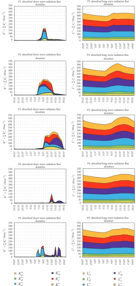
Figure 6 illustrates the short- and longwave radiation flux densities absorbed by a standing or walking “reference person” (𝐾∗𝑖,𝐿∗𝑖), a typical subject usually assumed in human- biometeorological studies in the case of𝑇mrtcalculations (𝐾𝑖∗
=𝑎𝑘× 𝑊𝑖× 𝐾𝑖;𝐿∗𝑖 =𝑎𝑙× 𝑊𝑖× 𝐿𝑖). The absorbed radiation components from the different directions are illustrated in a cumulative way to indicate the sum of absorbed short- and longwave radiation energy, that is, the short- and longwave radiation loads as well (𝐾∗,𝐿∗). Moreover, the same ordinate was adopted in the case of each short- and longwave graphical chart-pair to allow easy and accurate comparison of their contributions to the resulting whole radiation income of the human body (and therefore their role in the resulted𝑇mrt).
At night, in the absence of solar radiation, the radiation budget consists of longwave components only. Although 𝐿∗𝑖 dominates daytime as well, the spatial and temporal differences in the whole radiation budget (and thus, in𝑇mrt) are primarily the result of the shortwave components (𝐾∗𝑖).
Due to the adopted directional-dependent weighting for a standing person, the influence of the vertical components (𝐾𝑢, 𝐾𝑑,𝐿𝑢, and𝐿𝑑) decreases greatly. That is, if a person crosses the area or walks on the sidewalks by the buildings, then his/her radiation load originates primarily from lateral directions: mostly from direct solar radiation (𝐾𝑒and/or𝐾𝑠 and/or𝐾𝑤) and from the emitted longwave radiation of the irradiated fac¸ades (𝐿𝑒,𝐿𝑠,𝐿𝑤, and𝐿𝑛).
Figure 6 indicates the observed differences in radiation loads between the five measurement locations. People have to face the greatest radiation load at P3 and P2 points owing to both the orientation of adjacent fac¸ades (ESE and SSW) and the lack of shade trees or any artificial devices. During the day, the summed𝐾∗ is considerably high for a rather long time at these points: at P2 the maximum of𝐾∗ is around 250 Wm−2(between 9:00 and 10:00), and at P3 the maximum 𝐾∗is around 280 Wm−2(between 14:00 and 15:00) with four hours over 250 Wm−2. Compared to𝐾∗,𝐿∗changes gradually with delayed peak values.𝐿∗ calculated for P2 reached its maximum around noon and exceeded 500 Wm−2 for two hours. In the case of P3,𝐿∗exceeded 500 Wm−2for over five hours, resulting in a maximum that extended over most of the afternoon. While𝐿∗values exceeding 450 Wm−2existed for about 8-9 hours at P2 and for 10 hours at P3, at other mea- surement locations𝐿∗only briefly reached this value in the afternoon. In the case of P1,𝐿∗remained considerably lower throughout the day. While low𝐾∗and𝐿∗values are primarily the result of the favorable NNE exposure of the P1 point, in the case of P4 and P5 the lower radiation income is the result of tree shading. It is worth emphasizing that with its WNW exposure, P4 would be subject to considerable radiation load over the afternoon if it would not be shaded by trees.
Figure 7 illustrates the obtained 𝑇mrt values (as a result of the above discussed conditions), the air temperature (𝑇𝑎) values and their differences (𝑇mrt− 𝑇𝑎) for each site. In terms of𝑇𝑎, there is little difference between the sites; during the
night, the values remain within a 0.5∘C range, whereas during the day, the greatest difference of 3∘C is observed between the warmest P3 and the coldest P1 point. In contrast,𝑇mrt differences between the five sites are much greater. In terms of𝑇mrt, P3 is the warmest with a maximum of 74∘C and with values over 70∘C for four hours in the afternoon. The daily maximum remained somewhat lower (68∘C) and occurred somewhat sooner in the case of P2. However, at P2 too, a prolonged, four-hour period with rather stressful conditions (values over 65∘C) can be observed in the afternoon. In contrast, 𝑇mrt at P1 remained below 30∘C for the whole afternoon. In the case of the three mostly shaded points (P1, P4, and P5) the𝑇mrtvalues were closer to𝑇𝑎and remained below 55∘C even during the short irradiated periods.
For most of the day, there is little difference between𝑇𝑎 and𝑇mrtat P1. In the case of P4,𝑇mrtexceeds𝑇𝑎by only a few degrees during the afternoon. At these points, the𝑇mrt− 𝑇𝑎 difference grew only to about 31∘C (P1) and 23∘C (P4) during the short periods of irradiation. As a result of direct solar radiation in the forenoon and the afternoon, the𝑇mrt − 𝑇𝑎 difference at P5 rose to the 20–30∘C interval. In contrast, during high solar angles when the crown provided sufficient protection, this difference remained around 5∘C. In the case of the most stressful locations (P2, P3),𝑇mrtexceeded𝑇𝑎by over 40∘C, conditions that persisted for about four hours.
3.2. Model Validation. Figure 8 presents the 𝑇mrt values obtained through the different models in comparison with the measurement-based ones and the course of𝑇mrtmodel errors (Δ𝑇mrt).Δ𝑇mrtvalues were calculated for each obser- vations site (P1–P5) and for each numerical model. 𝑇mrt model errors were greater during the daytime than at night.
Greater deviations from measured values generally occurred around sunrise and sunset because of differences in model resolutions. A good example to this error is the period from around 6:00 to 7:00 at P1, P2, and P3 sites. Here, ENVI-met (the coarsest model with 3 m×3 m×0.5 m resolution) lags behind SOLWEIG and RayMan Pro. To facilitate the visual analysis, the time of sunrise (SR) and sunset (SS), as well as the periods of direct solar radiation, are indicated at the bottom of each graph (Figure 8).
In general, extreme deviations (i.e., peaks and valleys) are the outcome of the mismatch between observed and modeled times when a given observation point becomes irradiated or shaded. A good example for this kind of error is the graph of P2. Here, ENVI-met’s error curve dips at 8:00 (indicating that the place is still shaded according to the model), but it rebounces by 9:00 in the morning. Similarly, when the observation point becomes shaded in the afternoon at around 14:00, each model still indicates the presence of direct radiation and hence significantly overestimates the actual 𝑇mrtvalues. Nevertheless, this extreme error disappears from the next observation in the following hour. These errors may arise either from coarse model resolutions or from differences between actual and modeled obstructing bodies (i.e., trees, buildings, or shading devices).
Besides the model-based errors (due to model inaccu- racies and coarse model resolutions) other modeling error trends can also be deduced from the results:
P1: absorbed short-wave radiation flux densities
21:07 23:07 1:07 3:07 5:07 7:07 9:07 11:07 13:07 15:07 17:07 19:07
19:07
P1: absorbed long-wave radiation flux densities
P2: absorbed short-wave radiation flux densities
5:22
3:221:22 7:22 9:22
21:22 23:22 11:22 13:22 15:22 17:22 19:22
19:22
P2: absorbed long-wave radiation flux densities
P3: absorbed short-wave radiation flux densities
21:37 23:37 17:3715:3713:3711:37 19:37
19:37 7:375:373:371:37 9:37 21:37 23:37 17:3715:3713:3711:37 19:3719:37 7:375:373:371:37 9:37
P3: absorbed long-wave radiation flux densities
L∗=∑L
∗ i−2(Wm)
P4: absorbed short-wave radiation flux densities
21:52 23:52 1:52 3:52 5:52 7:52 9:52 11:52 13:52 15:52 17:52 19:52
19:52 21:52 23:52 1:52 3:52 5:52 7:52 9:52 11:52 13:52 15:52 17:52 19:5219:52
P4: absorbed long-wave radiation flux densities
P5: absorbed short-wave radiation flux densities
P5: absorbed long-wave radiation flux densities
K∗u K∗d K∗e
Kw∗ Ks∗ Kn∗
L∗u L∗d L∗e
L∗w L∗s L∗n
L∗=∑L
∗ i−2(Wm) 0
50 100 150 200 250 300 350 400 450 500 550
K∗=∑K
∗ i
L∗=∑L
∗ i
0 50 100 150 200 250 300 350 400 450 500 550
1:22 3:22
21:22 23:22 5:22 7:22 13:2211:22 15:22 17:229:22 19:22
19:22
0 50 100 150 200 250 300 350 400
K∗=∑K
∗ i−2(Wm) 450500
550
0 50 100 150 200 250 300 350 400 450 500 550
0 50 100 150 200 250 300 350 400
K∗=∑K
∗ i−2(Wm) 450 500 550
0 50 100 150 200 250 300 350 400
L∗=∑L
∗ i−2(Wm) 450 500 550
0 50 100 150 200 250 300 350 400
K∗=∑K
∗ i−2(Wm ) 450
500 550
0 50 100 150 200 250 300 350 400 450 500 550
0 50 100 150 200 250 300 350 400
K∗=∑K
∗ i−2(Wm) 450 500 550
0 50 100 150 200 250 300 350 400
L∗=∑L
∗ i−2(Wm) 450 500 550
(Wm−2) (Wm−2) 17:0711:073:07 7:07 9:0723:07 13:07 19:0719:07 15:071:0721:07 5:0721:07 11:071:07 3:07 5:07 7:07 9:07 15:07 17:0723:07 13:07 19:0719:07
Figure 6: Sum of the short- (𝐾𝑖∗) and longwave (𝐿∗𝑖) radiation flux densities absorbed by the standing reference person at the five survey points (𝑎𝑘: 0.7,𝑎𝑙: 0.97,𝑊𝑖: 0.06 for vertical directions and 0.22 for lateral directions).
P1: air emperature & mean radiant temperature
−10 0 10 20 30 40 50 60 70 80
Ta,Tmrt,(Tmrt−Ta) [∘ #] 21:00 0:00 3:00 6:00 9:00 12:00 15:00 18:00 21:0018:00
P2: air emperature & mean radiant temperature
−10 0 10 20 30 40 50 60 70 80
Ta,Tmrt,(Tmrt−Ta) [∘ #] 21:00 0:00 3:00 6:00 9:00 12:00 15:00 18:00 21:0018:00
P3: air emperature & mean radiant temperature
21:00 0:00 3:00 6:00 9:00 12:00 15:00 18:00 21:00
18:00
−10 0 10 20 30 40 50 60 70 80
Ta,Tmrt,(Tmrt−Ta) [∘ #]
P4: air emperature & mean radiant temperature
−10 0 10 20 30 40 50 60 70 80
Ta,Tmrt,(Tmrt−Ta) [∘ #] 21:00 0:00 3:00 6:00 9:00 12:00 15:00 18:00 21:0018:00
P5: air emperature & mean radiant temperature
−10 0 10 20 30 40 50 60 70 80
Ta,Tmrt,(Tmrt−Ta) [∘ #] 21:00 0:00 3:00 6:00 9:00 12:00 15:00 18:00 21:0018:00
Ta Tmrt
Tmrt− Ta
Figure 7: Air temperature (𝑇𝑎), mean radiant temperature (𝑇mrt), and their differences at the five survey points.
(i) First, all models underestimate nighttime 𝑇mrt by 5–10∘C—except for SOLWEIG, in cases of sites that mostly remain shaded by trees (P4, P5).
(ii) Second, for those daylight hours when the survey points were shaded by buildings for a long time 𝑇mr is generally overestimated by ENVI-met and SOLWEIG, whereas RayMan Pro hovers near or just below zero (P1, P4). For those daylight hours when the survey points were shaded by trees we can deduce similar trends, except for RayMan at P5. (At P5 𝑇mr is greatly overestimated by RayMan as a result
of a subsequently discovered model glitch in which the modeled tree above the observation point lacks its crown. Although the imported obstacle file was correct, authors were not able to fix this unusual bug of RayMan in the case of this point).
(iii) Third, all models underestimate the daytime 𝑇mrt when the observation points became irradiated by the sun and this is especially true for RayMan. In our validation, SOLWEIG and ENVI-met performed better in modeling the radiative conditions in these complex urban environments.
21:00 6:00 9:00 12:0015:00 18:00 21:00
18:00
P1
3:00
0:00
0 10 20 30 40 50 60 70 80
Tmrt∘ C))
Night Short-time
insolation Building shade
SS SR SS
P1
21:00 0:00 3:00 6:00 9:00 12:00 15:00 18:00 21:00
18:00
−40
−30
−20
−10 0 10 20 30
ΔTGLN(∘ C) (modeled−measured) 40
Night Short-time
insolation Building shade
SS SR SS
0 10 20 30 40 50 60 70 80
TGLN(∘C) 21:00 0:003:00 6:00 9:00 12:0015:00 18:00 21:0018:00
P2
Night Building
shade Unobstructed insolation
SS SR SS
P2
−40
−30
−20
−10 0 10 20 30 40
ΔTGLN(∘ C) 21:00 0:00 3:00 6:00 9:00 12:00 15:00 18:00 21:0018:00
(modeled−measured)
Night Building
shade Unobstructed insolation
SS SR SS
P3
21:00 0:003:00 6:00 9:00 12:0015:00 18:00 21:00
18:00
0 10 30 20 40 50 60 70 80
TGLN(∘ C)
Night Building
shade Unobstructed insolation
SS SR SS
−40
−30
−20
−10 0 10 20 30 40
ΔTGLN(∘C)
P3
21:00 0:00 3:00 6:00 9:00 12:00 15:00 18:00 21:00
18:00
(modeled−measured)
Night Building
shade Unobstructed insolation
SS SR SS
P4
0 10 20 30 40 50 60 70 80
TGLN(∘C) 21:00 0:003:00 6:00 9:00 18:00 21:0018:00 15:0012:00
Night Building shade Tree shade
Short-time insolation
SS SR SS
P4
ΔTGLN(∘C) 21:00 0:003:00 6:00 9:00 18:00 21:0018:00
(modeled−measured)
−40
−30
−20
−10 0 10 30 20 40
15:00
12:00
Night Building shade Tree shade Short-time insolation
SS SR SS
P5
0 10 20 30 40 50 60 70 80
TGLN(∘ C) 21:00 0:00 3:00 6:00 9:00 12:00 15:00 18:00 21:0018:00
Measured ENVI-met
SOLWEIG
RayMan
Tree shade Night
Short insolation periods
Short insolation periods
SS SR SS
P5
−40
−30
−20
−10 0 10 20 30 40
ΔTGLN(∘ C) 21:00 0:00 3:00 6:00 9:00 12:00 15:00 18:00 21:0018:00
(modeled−measured)
ENVI-met - Measured SOLWEIG -Measured RayMan - Measured
Tree shade Night
Short insolation
periods Short insolation periods
SS SR SS
Figure 8: Deviation of the modeled𝑇mrtvalues from the measurement-based𝑇mrtat the five points during the survey period (SS: sunset, SR:
sunrise; note: data are calculated from 15-minute averages). Horizontal bars at the bottom of each graph indicate when the measurement point became shaded or exposed to the sun as follows: (i) yellow and orange colors mark shorter and longer periods of solar exposure, respectively;
(ii) light green indicates period of shade from trees; (iii) dark green suggests shade from buildings; (iv) dark gray signals nighttime with no short-wave radiation. SS and SR marks indicate times of sunset and sunrise, respectively.