Modell alapú diagnosztikai módszerek energetikai alkalmazásokkal

methods with energetic applications

DOI:10.18136/PE.2020.754

PhD Thesis

Author: Anna Ibolya Pózna

Supervisors: Katalin Hangos, DSc Miklós Gerzson, CSc

University of Pannonia Faculty of Information Technology Doctoral School of Information Science

Veszprém 2020

Értekezés doktori (PhD) fokozat elnyerése érdekében Írta:

Pózna Anna Ibolya

Készült a Pannon Egyetem Informatikai Tudományok Doktori Iskolájának keretében

Témavezet®k:

Dr. Hangos Katalin

Elfogadásra javaslom: igen / nem

aláírás Dr. Gerzson Miklós

Elfogadásra javaslom: igen / nem

aláírás A jelölt a doktori szigorlaton ... %-ot ért el.

Az értekezést bírálóként elfogadásra javaslom:

Bíráló neve: ... : igen / nem

aláírás Bíráló neve: ... : igen / nem

aláírás A jelölt az értekezés nyilvános vitáján ... %-ot ért el.

Veszprém, ...

a Bíráló Bizottság elnöke

A doktori (PhD) oklevél min®sítése: ...

Acknowledgements 1

Abstract 2

1 Introduction 5

1.1 Background and motivation . . . 5

1.2 Model based diagnosis in dynamic systems . . . 6

1.2.1 Diagnosis based on parameter estimation . . . 6

1.2.2 Diagnosis based on analytical redundancy . . . 7

1.2.3 Diagnosis of discrete event systems . . . 8

1.3 Thesis structure . . . 9

2 Diagnosis of batteries using parameter estimation 11 2.1 Battery basic notions . . . 12

2.2 Battery model . . . 14

2.2.1 Modelling assumptions . . . 14

2.2.2 Temperature dependent battery model . . . 14

2.3 Experiment design . . . 18

2.3.1 Parameter sensitivity analysis . . . 19

2.3.2 Input signal . . . 21

2.3.3 Simulation setup . . . 21

2.4 Methods for parameter estimation . . . 22

2.4.1 Estimation of the battery parameters . . . 23

2.4.2 Estimation of the temperature dependency of the pa- rameters . . . 23

2.5 Simulation results . . . 24

2.5.1 Estimated battery parameters . . . 25

2.5.2 Estimated temperature dependent parameters . . . 31

2.6 Discussion and future work . . . 32

2.7 Summary . . . 33

3 Model based diagnosis of electrical networks 34 3.1 Electrical network models, basic assumptions . . . 36

3.1.1 The model of the electrical network . . . 36

3.1.2 Technical and non-technical losses . . . 38

3.1.3 Measurements . . . 39

3.1.4 Notations . . . 39

3.2 Decomposition of electrical networks . . . 40

3.2.1 Basic structures of electrical networks . . . 40

3.2.2 The decomposition method . . . 42

3.2.3 Simple examples . . . 46

3.3 Diagnosis of electrical networks . . . 51

3.3.1 The principle of the method . . . 51

3.3.2 Fault detection and isolation for the one feeder radial layout . . . 57

3.3.3 Fault detection and isolation for the two feeder layout . . 60

3.4 Discussion and future work . . . 64

3.5 Summary . . . 66

4 Colored Petri net based diagnosis of process systems 67 4.1 Basic notions . . . 68

4.1.1 Qualitative range sets, events, traces and deviations . . . 68

4.1.2 Petri nets . . . 70

4.1.3 Colored Petri nets . . . 72

4.2 Colored Petri net model of process systems . . . 75

4.2.1 Modelling assumptions . . . 76

4.2.2 The structure of the CPN model . . . 76

4.2.3 The operation of the CPN model . . . 79

4.2.4 Generating the occurrence graph . . . 81

4.2.5 Multiple faults, faults on the y . . . 82

4.3 Unit-wise diagnosis . . . 82

4.3.1 Diagnosis using the occurrence graph . . . 82

4.3.2 The diagnostic algorithm . . . 83

4.4 Diagnosis with structural decomposition . . . 86

4.4.1 Composite systems . . . 87

4.4.2 Structural decomposition . . . 88

4.5 Discussion and future work . . . 90

4.6 Summary . . . 92

5 Theses 94 5.1 Thesis 1 - Parameter estimation method for temperature depen- dent battery parameters (Chapter 2) . . . 94

5.2 Thesis 2 - Non-technical loss diagnosis in electrical networks (Chapter 3) . . . 95

5.3 Thesis 3 - Colored Petri net based diagnosis of technological systems (Chapter 4) . . . 96

5.4 Related publications . . . 96

Appendix 98 A Case study of model based diagnosis of electrical networks . . . 98

A.1 Electrical network and its decomposition . . . 98

A.2 Diagnosis of the illegal users . . . 100 B Case study of colored Petri net based diagnosis of process systems104

Bibliography 109

First of all, I wish to express my deepest gratitude to my supervisors, Prof. Katalin Hangos and Dr. Miklós Gerzson, who convincingly guided and encouraged me to be professional and do the right thing even when the road got tough. Without their persistent help, the goal of this project would not have been realized.

I am also grateful to my colleagues Dr. Attila Magyar and Roland Bálint to their continuous support and companionship.

Furthermore I wish to thank to the members of the Department of Electrical Engineering and Information Systems for their encouragement through the years.

Finally I am grateful to my sisters Dia and Melinda, and my signicant other András who have provided emotional support during my work. I am also grateful to my other family members and friends who have supported me along the way.

Electrical energy is one of the most essential resources of the modern world.

Electrical energy systems usually have distributed structures with redundant and recongurable elements, which grant the safe and reliable operation of the system. The diagnosis of such a system is important because the failure of a component has eect on the fault tolerance of the whole system. Eective di- agnosis methods may reduce the number of equipments and save maintenance costs of a complex system. In this work dierent kinds of model based di- agnostic solutions are presented focused on energetic application areas, where the electrical energy system is modelled and analyzed at dierent levels of hierarchy.

First a parameter estimation method of batteries is presented, that can be a basis of a diagnostic method. A simple parametric temperature dependent battery model is used for this purpose. A two-step method is used that includes a parameter estimation step of the key parameters at dierent temperatures followed by a static optimization step that determines the temperature coe- cients of the corresponding parameters. The proposed method can be used as a computationally eective way of determining the key battery parameters at a given temperature, that can be used for battery health diagnosis.

Next, a diagnostic method is proposed for detecting and isolating non- technical losses (illegal loads) in low voltage electrical grids. The proposed method uses a simple static linear model of the network and it is based on analyzing the dierences between the measured and model-predicted voltages.

As a preliminary step of the diagnosis, the decomposition of the network is proposed to make the computation ecient. The uncertainty in the model parameters and measurements are also taken into account to make the ap- proach applicable in real-world cases. The proposed method is able to localize multiple illegal loads in the network.

At last a new on-line fault identication method of technological processes is proposed that uses a qualitative dynamic model of the system and its colored Petri net model. The diagnosis is based on searching the deviations between the traces of the normal and the actual operation on the occurrence graph of the model. In case of composite systems the occurrence graph can be ex- tremely large, therefore a structural decomposition method is applied which can manage increased computational eort and searching-time.

The presented methods can be applied in dierent areas of electrical sys- tem diagnosis. The battery parameter estimation method can be used for estimating battery age and remaining life, the available capacity and state of charge at dierent temperatures. The decomposition based methods can be

A villamos energia napjaink egyik meghatározó energiaforrása. A fogyasz- tók biztonságos és folyamatos ellátása érdekében, a villamos energetikai rend- szerek általában elosztott struktúrájú, számos redundáns illetve rekongurál- ható elemet tartalmazó rendszerek. A diagnosztika egy ilyen rendszerben nagy szerepet kap, mivel az egyes komponensek meghibásodása a teljes rendszer hibat¶r® képességét is befolyásolja. Hatékony diagnosztikai módszerek segít- ségével a berendezések száma és a karbantartási költségek optimalizálhatók.

Jelen értekezésben különböz® modell alapú diagnosztikai módszerek kerülnek bemutatásra, amelyek villamos energetikai rendszerek különböz® szint¶ vizs- gálatához kapcsolódnak.

El®ször egy akkumulátorok paraméterbecslésére szolgáló módszer kerül be- mutatásra, ahol az akkumulátor m¶ködését egy egyszer¶ parametrikus, h®- mérsékletfügg® modell írja le. A javasolt kétlépéses paraméterbecslési mód- szer segítségével az akkumulátor paraméterei és paraméterek h®mérséklet- függ® karakterisztikái hatékonya megbecsülhet®k. A módszer felhasználható akkumulátor-diagnosztikai alkalmazásokban, ahol az akkumulátor elhasználó- dottságára, élettartamára kell következtetni.

Ezután egy, a villamos hálózatokban jelen lév® nem mért vételezés diag- nosztikájára szolgáló módszer kerül bemutatásra. A módszer segítségével de- tektálni és azonosítani lehet a hálózatban jelen lév® illegális fogyasztókat. A javasolt diagnosztikai módszer pedig a mért és a hálózat statikus lineáris mo- dellje által jósolt feszültségek és áramok összehasonlításán alapul. A kifejlesz- tett módszer egyszerre több illegális fogyasztó azonosítására is képes, valamint gyelembe veszi a hálózat paramétereinek bizonytalanságát, és a mérési hi- bákat is. A módszer hatékonyságának növelése érdekében a hálózat el®zetes dekompozíciója javasolt.

Végül technológiai rendszerek kvalitatív modell alapú diagnosztikája kerül ismertetésre. A diagnosztikai módszer a technológiai rendszer normál és hibás m¶ködéseit leíró eseménysorai közötti eltérések vizsgálatán alapszik, felhasz- nálva a rendszer színezett Petri háló modelljének elérhet®ségi gráfját. Összetett rendszerek diagnosztikája esetében a rendszer el®zetes strukturális dekompozí- ciója javasolt, a különböz® egységekben el®forduló hibák könnyebb azonosítása érdekében.

A bemutatott módszerek különböz® területeken alkalmazhatóak. Az ak- kumulátor paramétereinek becslése felhasználható az aktuális és a hátralév®

élettartam, az elérhet® kapacitás és töltöttségi szint becslésére különböz® h®- mérsékleteken. A dekompozíció alapú módszerek statikus és dinamikus mo- dellek esetében is alkalmazhatóak. Ezen kívül a dekompozíció lehet®vé teszi, hogy többszörös hibák is könnyen azonosíthatóak legyenek, valamint a számí- tási igényt is kedvez®en befolyásolja.

Ýëåêòðè÷åñêàÿ ýíåðãèÿ îäèí èç ñàìûõ âàæíûõ ðåñóðñîâ ñîâðåìåí- íîãî ìèðà. Ñèñòåìû ýëåêòðè÷åñêîé ýíåðãèè îáû÷íî èìåþò ðàñïðåäåëåí- íûå ñòðóêòóðû ñ ìíîãèìè èçáûòî÷íûìè ýëåìåíòàìè, êîòîðûå îáåñïå÷è- âàþò áåçîïàñíóþ è íàä¼æíóþ ðàáîòó ñèñòåìû. Äèàãíîñòèêà òàêèõ ñèñòåì î÷åíü âàæíàÿ, ïîòîìó ÷òî ïîâðåæäåíèå îäíîãî ýëåìåíòà âëèÿåò íà îòêà- çîóñòîé÷èâîñòü âñåé ñèñòåìû. Ýôôåêòèâíûå ìåòîäû äèàãíîñòèêè ìîãóò óìåíüøèòü êîëè÷åñòâî îáîðóäîâàíèé è ðàñõîäû íà òåõíè÷åñêîå îáñëóæè- âàíèå ñëîæíûõ ñèñòåì.  ýòîé äèññåðòàöèè ïðåäñòàâëÿþòñÿ ðàçíûå âèäû äèàãíîñòèêè íà îñíîâå ìîäåëè ýíåðãåòè÷åñêèõ ñèñòåì.

Ñíà÷àëà ïðåäñòàâëÿåòñÿ ìåòîä îöåíêè ïàðàìåòðîâ àêêóìóëÿòîðà, êîòî- ðûé ìîæåò áûòü îñíîâà ìåòîäà äèàãíîñòèêè. Äëÿ ýòîé öåëè èñïîëüçîâàíà ïðîñòàÿ ìîäåëü àêêóìóëÿòîðà, çàâèñèìàÿ îò òåìïåðàòóðû. Ðàçðàáîòàííûé ìåòîä ñîñòîèò èç äâóõ ýòàïîâ. Íà ïåðâîì ýòàïå îöåíèâàþòñÿ êëþ÷åâûå ïà- ðàìåòðû àêêóìóëÿòîðà ïðè ðàçíûõ òåìïåðàòóðàõ. Íà âòîðîì ýòàïå îöå- íèâàþòñÿ òåìïåðàòóðíûå êîýôôèöèåíòû ïàðàìåòðîâ ñ ïîìîùüþ ñòàòè÷å- ñêîé îïòèìèçàöèè. Ïðåäëîæåííûé ìåòîä ìîæíî èñïîëüçîâàòü êàê âû÷èñ- ëèòåëüíî ýôôåêòèâíûé ñïîñîá, ÷òîáû îöåíèòü ïàðàìåòðû àêêóìóëÿòîðà.

Ïîñëå ýòîãî, ïðåäñòàâëÿåòñÿ äèàãíîñòè÷åñêèé ìåòîä äëÿ äåòåêòèðîâà- íèÿ è èçîëÿöèè íåòåõíè÷åñêèõ ïîòåðü â ýëåêòðè÷åñêèõ ñåòÿõ. Äëÿ ýòîé öå- ëè èñïîëüçîâàíà ñòàòè÷åñêàÿ ëèíåàðíàÿ ìîäåëü ýëåêòðè÷åñêîé ñåòè. Ïðåä- ëîæåííûé ìåòîä îñíîâûâàåòñÿ íà àíàëèçå èçìåðåííûõ è ïðåäñêàçàííûõ íàïðÿæåíèé. Äëÿ òîãî ÷òîáû ñäåëàòü ìåòîä âû÷èñëèòåëüíî ýôôåêòèâ- íûì, ïåðåä äèàãíîñòèêîé ïðåäëàãàåòñÿ äåêîìïîçèöèÿ ñåòè. Ðàçðàáîòàí- íûé äèàãíîñòè÷åñêèé ìåòîä ìîæåò ëîêàëèçîâàòü íåñêîëüêî íåëåãàëüíûõ ïîòðåáèòåëåé, ó÷èòûâàÿ ïîãðåøíîñòè èçìåðåíèÿ.

Íàêîíåö, ïðåäëàãàåòñÿ íîâûé îíëàéí ìåòîä äèàãíîñòèêè òåõíîëîãè÷å- ñêèõ ïðîöåññîâ êîòîðûé èñïîëüçóåò êà÷åñòâåííóþ äèíàìè÷åñêóþ ìîäåëü ñèñòåìû â ôîðìå öâåòíîé ñåòè Ïåòðè.  ýòîì ñëó÷àå äèàãíîñòèêà îñíî- âûâàåòñÿ íà ïîèñêå ðàçíèö ìåæäó ñëåäàìè íîðìàëüíîé è ðåàëüíîé îïåðà- öèè íà ãðàôå äîñòèæèìîñòè. Ãðàôû äîñòèæèìîñòè ñëîæíûõ ñèñòåì ìîãóò áûòü îãðîìíûìè, ïîýòîìó ïðåäëàãàåòñÿ ìåòîä ñòðóêòóðíîé äåêîìïîçèöèè, êîòîðûé ìîæåò óïðàâëÿòü ïîâûøåííûìè âû÷èñëèòåëüíûìè óñèëèÿìè è âðåìåíåì íà ïîèñê.

Ïðåäñòàâëåííûå ìåòîäû ìîãóò ïðèìåíÿòüñÿ â ðàçëè÷íûõ îáëàñòÿõ äè- àãíîñòèêè ýëåêòðè÷åñêèõ ñèñòåì. Ìåòîä îöåíêè ïàðàìåòðîâ àêêóìóëÿòî- ðà ìîæåò èñïîëüçîâàòüñÿ äëÿ îöåíêè ñðîêà ñëóæáû, åìêîñòè èëè óðîâ- íÿ çàðÿäà àêêóìóëÿòîðà ïðè ðàçíûõ òåìïåðàòóðàõ. Ìåòîäû, îñíîâàííûå íà äåêîìïîçèöèè, ìîãóò èñïîëüçîâàòüñÿ äëÿ äèàãíîñòèêè è ñòàòè÷åñêèõ è

Introduction

1.1 Background and motivation

Electrical energy plays a fundamental role in our everyday life. Industrial processes, communication, household tasks, entertainment or transportation in modern days would be inconceivable without electrical energy. The transmis- sion of the electrical energy from the place of generation to the consumption requires complex and extensive transmission and distribution networks, which may even go beyond country borders. Therefore, research done in the area of these transmission and distribution networks and their elements (electrical machines, consumption equipments, batteries, power sources etc.), called as electrical energy systems, are of great importance.

Electrical energy systems are usually distributed systems with high degree of redundancy and recongurability. To grant the continuous operability of the system and the availability of the energy, electrical energy systems are usually equipped with backup systems therefore a single fault should not signicantly aect the operation of the system. The diagnosis of the system components is important because it aects the fault tolerance of the whole system. An eective diagnostic method may reduce the number of necessary redundant components and additional costs of (e.g. maintenance). Therefore the diag- nosis of electrical energy systems is crucial for the maintainers, operators and customers of the system.

The diagnosis of the electrical energy systems can be performed at dierent levels with dierent capabilities. Sometimes it is only enough to detect the presence of the fault, but usually the type and the location of the occurred fault should be identied. The situation may become even more complicated if there are multiple faults in the system. Moreover an other advantage of the model based diagnosis is that the model used for the diagnosis can be utilized in other areas of the investigation of the system (e.g. verication).

Electrical energy systems can be modelled and analyzed at dierent levels of hierarchy. At the top level network model a simple static linear model may be enough to describe the main operation of the network [1]. Going down to lower levels, such as distribution networks, local low-voltage networks, consumers and devices, the models of the components become more complex and detailed and oer higher resolution in space and time [2]. For example a local network can be modelled as a discrete event system [3]; or a low level

component, like a battery can be modelled by a nonlinear state space model [4]. When modelling a certain part of the network one selects the appropriate model type according e.g. to the modelling goal, the targeted application area and the available computational resource.

In this work various model based fault diagnostic methods applied to elec- trical energy systems are presented with dierent approaches of the diagnostic task. The presented methods vary in the applied method, the used system model and the application area.

1.2 Model based diagnosis in dynamic systems

Each system has an expected way of operation that satises the purpose for which it was created. However it can sometimes occur that the system op- erates incorrectly because of dierent reasons. The malfunction of the system can be caused by a fault. The sign of the fault is the deviation between the ac- tual (measured, observed or computed) and the nominal variables/parameters, that is called error. If the error remains unnoticed and the fault is not handled properly, then the situation may lead to the failure of the system. A failure occurs when the system can no longer satisfy its original function, or its per- formance is degraded [5]. Faults may change the structure, variables or the parameters of the system model [6]. Model based diagnosis is one of the most popular group of diagnostic methods [7].

The general diagnostic task can be described in the following way [8].

Given a set of faults F (where f₀ ∈ F refers to the faultless mode), a dy- namic system model including the possible fault models and the measured input-output data: U = (u(0), u(1), . . . , u(k)), Y = (y(0), y(1), . . . , y(k)). The diagnostic task is to nd the faultf for a given input-output pair(U, Y).

Dierent levels of the diagnosis can be distinguished based on the depth of resolution. The task of fault detection is to decide whether any fault has occurred in the system or not. Fault isolation aims to determine the location of the fault within the system. Fault identication is used to determine exactly which fault in F has occurred and estimate its magnitude.

In the following a short review of model based diagnostic methods that are used in this thesis is given.

1.2.1 Diagnosis based on parameter estimation

The basic principle of the method is that the occurrence of a fault makes changes in the variables or parameters of the system. Given the set of faults,

Several methods of parameter estimation can be used to solve this task.

One of the most popular methods is the least squares estimation and its vari- ations because of their simplicity.

The parameter estimation based diagnosis is usually applied at component level because of the complexity of the model and the number of parameters.

In [10] a parameter estimation based fault detection method was developed for a DC motor where both electrical and mechanical parameters were estimated.

Recursive least squares are often used for real-time diagnosis exploiting the reduced computational eort [11]. Nonlinear weighted least squares was used to predict the degradation of a gas turbine [12]. Parameter estimation can also be a part of a hybrid diagnoser as it was applied in [13], [14].

The parameter estimation methods can be applied with high reliability only if the input is properly excited. Experiment design aims to create op- timal conditions for parameter estimation. The papers [15] and [16] propose an experiment design solution that is optimal from the parameter identica- tion point of view, where solution space is a sinusoidal signal family applied as charging/discharging current. On the other hand, experiment design [17]

can also be used in order to maximize the information content of the battery charging-discharging related measurement dataset in order to estimate battery parameters more precisely.

Parameter estimation of nonlinear models can be computationally complex since the loss function should be minimized numerically. Paper [18] overcomes this problem by a parallel Java algorithm implemented on GPU (CUDA) archi- tecture. The authors of [19] developed and compared three dierent solutions for the internal resistance estimation of lithium-ion batteries (direct resistance estimation, Extended Kalman Filter (EKF), recursive Least Squares) and con- cluded that EKF approach performed the best in terms of computational e- ciency.

The advantage of the parameter estimation based diagnosis is that all fault diagnosis tasks (detection, isolation, identication) can be realized with this method. Besides that, with on-line parameter estimation methods faults can be recognized at an early stage and the detection of multiple faults is also possible.

1.2.2 Diagnosis based on analytical redundancy

Analytical redundancy based diagnosis methods use the idea that the actual measured variables should be consistent with the model calculated variables [20]. Analytical redundancy relations (ARR) are equations representing the deviations between the measured and model variables that are zero in case of normal operation and nonzero in case of at least one fault.

Analytical redundancy based diagnosers usually have two components. The residual generator computes the the dierence between measured and model variables (residuals). Usually three dierent approaches are used for residual generation: the parity space, the observer and the Kalman lter methods. The decision system analyzes the residuals and complete the fault detection and isolation tasks [21].

The fault detection task is relatively simple with analytical redundancy.

However the residuals being zero in/during normal operation is typically not true in real world applications because of the presence of measurement noise.

Therefore the residuals are usually compared to a given threshold to detect faults in the system[22]. When the measurement noise is signicant then in- formation about the noise should be included in the model. Using a properly designed lter the eect of noise can be attenuated.

For fault isolation more than one residual is needed. The two main isola- tion techniques that can be used are the method of structured residuals and the xed direction residuals [23]. In the rst case the residuals can be divided into subsets that are nonzero only if a specic fault has occurred. The pattern of zero and nonzero elements of the residuals, which is called signature, char- acterizes the fault. In the second case the direction of the residual vector can be associated with the given fault.

Analytical redundancy is often used to diagnose sensor or actuator faults.

Application areas range from simple benchmark systems like the three tank system in [24] to complex engineering systems and safety critical systems such as nuclear power plants [25], jet engines [26], satellites [27] or aerospace [28].

The advantage of analytical redundancy based diagnosis in contrast to hardware redundancy is that no duplication of sensors or physical components is needed to realize a diagnostic method. This reduces the cost and weight of the equipment. An other feature is that a variety of models can be served as the basis of the diagnosis (e.g.ordinary dierential equations, data-driven models, expert systems) [29].

1.2.3 Diagnosis of discrete event systems

Discrete event systems are special kinds of dynamic systems with discrete time and discrete valued variables. Events are the changes between the discrete values of the variables. Typical models of discrete event systems are automata models and their extensions, Petri nets or state machines.

Fault diagnosis of discrete event systems is usually based on the assumption that faults are unobservable events, therefore only the eects of faults can be noticed [30]. Since events related to faults are unobservable by assumption,

If the discrete event system is modelled by an automaton then the most common solution of the diagnostic problem is the creation of the diagnoser au- tomaton by eliminating the unobservable events. Although the diagnoser can be constructed algorithmically, the issues of state explosion and high compu- tational complexity are present. A solution to reduce the computational eort was presented in [32].

Another way of diagnosis is performed by checking the consistency of the observed input-output sequences and the state transition relations of the au- tomaton model [33]. The method can be applied to quantised systems repre- sented by discrete event models, too [34].

Discrete event systems can be represented by dierent kinds of Petri nets, too. A simple fault detection method based on the measurement of token quantity in conservative Petri nets is given in [35]. In case of more complex models more sophisticated diagnostic methods are needed. The construction of a diagnoser Petri net, which is the copy of the original model without the faulty transitions, is proposed in [36], [37]. Comparing the original model output and the diagnoser output the dierence between them indicates that a fault has occurred. Besides that, the reachability or the coverability graph of the Petri net is often used for diagnostic purposes, because it contains all possible system states [38]. Other methods use the mathematical model of the Petri net and the diagnostic problem is traced back to the solution of a set of linear equations [39], [40]. Qualitative discrete event systems, which is in the focus of Chapter 4, can be also modelled by ordinary or colored Petri nets [41], [42]. The trace of the qualitative variables can be used for detecting and identifying faults in the system, using a specially constructed colored Petri net diagnoser [43].

The problems of the Petri net based diagnostic methods are similar to the ones mentioned at the automata based methods.

1.3 Thesis structure

This thesis is divided into the following main chapters.

In Chapter 2 the parameter estimation method developed for the diagnosis of batteries is presented. First the basic notions related to the battery op- eration are introduced then the used temperature dependent battery model is introduced. After that the experiment design process that is a necessary prerequisite of the parameter estimation is described. The developed two-step parameter estimation method is explained hereinafter. Finally, simulation re- sults are presented and the achieved results are summarized.

In Chapter 3 the model based diagnosis of electrical networks is described which is based on the comparison of nominal and measured current/voltage values. First the model of the network and the basic concepts are introduced.

Then the decomposition of dierent network structures is presented which is

the key element of the diagnostic method. After that the proposed diagnos- tic algorithms for non-technical loss diagnosis utilizing the network structures are presented. The decomposition and diagnostic methods are illustrated on simple examples. The results are summarized at the end of the chapter.

In Chapter 4 the colored Petri net based diagnostic method for process systems is presented. At rst the basic notions of ordinary and colored Petri nets are introduced. The general colored Petri net model and its operation is explained in the next section. After that the basic unit-wise diagnostic algorithm is presented which uses the occurrence graph of the colored Petri net model of the technological unit. The diagnosis of composite systems based on structural decomposition is introduced in the next section. Finally, the results of this work are summarized.

In Chapter 5 the main results of this research are summarized in three thesis points. The relevant publications can also be found here.

Two detailed case studies illustrating the diagnostic methods presented in Chapter 3 and Chapter 4 can be found in the Appendix.

Diagnosis of batteries using parameter estimation

Lithium-ion batteries are popular energy sources of our everyday life be- cause of their high energy density, low self-discharge and light weight. Portable electronic devices (mobile phones, laptops), home electronics, electronic tools and electric vehicles (EVs) all run on some type of lithium-ion battery. In ap- plications like electrical vehicles, batteries are connected in parallel and series in order to meet the power needs.

The optimal performance and safe operation of the set of battery cells are managed by the battery management system (BMS). Another essential role of the BMS is the state of charge (SOC) and state of health (SOH) estimation.

The former quantity informs the user on the remaining charge of the battery bank (i.e. the remaining mileage that can be travelled with the electrical vehicle), while the latter shows the ratio between the capacity of a new battery in relation to the actual capacity of the battery. Just like any other battery, the performance of the lithium-ion battery is not constant but slowly degrades during the operation and strongly depends on the ambient temperature. The battery health conditions cannot be measured directly therefore it should be estimated based on measurable quantities.

The temperature does not only aect the aging process of a battery but its short term performance, too. Therefore the thermal eects taking place in the battery should also be taken into account when creating a battery model.

Thermal modelling and the analysis of lithium-ion batteries under dierent temperatures has been addressed by several authors. The thermal modelling of batteries as well as the modelling without temperature dependency can be classied based on the scientic background (e.g. equivalent circuit models, electrochemical models). The review [44] gives a thorough analysis not only of the dierent electrochemical models but also of the parameter identication methods.

In such applications where the computational complexity (i.e. time) is crucial e.g. in BMSs, equivalent circuit models are widely used [45]. In our previous work [46] we proposed a parameter estimation for lithium ion batteries based on their rst order equivalent circuit model. The results showed that there is a linear dependency between some model parameters because of the insucient excitation.

The aim of the work presented here is to diagnose the failure of the battery related to the aging. Because the aging process aects the battery parameters (e.g. decreased capacity), the condition of the battery can be estimated by comparing the actual battery parameters with the parameters of a new bat- tery. To do this the actual battery parameters should be determined. In the following sections I propose a parameter estimation method which takes into account the temperature dependency of the parameters, too. The tempera- ture dependent battery operation is critical in automotive applications (e.g.

the available charge in a battery at 0^◦C is less than at 25 ^◦C).

In this chapter I generalize my previous work to the case when the tem- perature dependence of the parameters are also taken into account. The way of estimation of the temperature dependent parameters is important from the viewpoint of applicability a simple parameter estimation is needed for primarily the actual capacity for implementation in future BMSs. In this work a dif- ferent equivalent circuit model is used instead of the one in [46], with physical meanings of the parameters. The novelty of this work is the two-step param- eter estimation method of the temperature dependent parameters. Before the estimation of the parameters, proper experiment design was carried out to ensure sucient excitation and maximize the available information about the parameters. The proposed method can be used as a basis of a battery health diagnosis system.

2.1 Battery basic notions

In this section the basic notions related to the operation of Li-ion batteries are summarized according to [47].

The battery is an electrochemical energy source that is composed of recharge- able cells. The battery delivers voltage that depends on the cell chemistry. The components of an electrochemical cell are the positive electrode , the negative electrode and the electrolyte. In case of Li-ion battery the positive electrode (cathode) is made from metal oxide, the negative electrode (anode) is made from carbon (graphite) and the electrolyte is a liquid solvent with lithium salt.

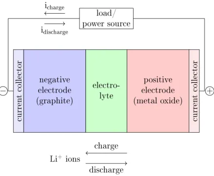
The schematic structure of a Li-ion battery can be seen in Figure 2.1.

Batteries have two operation modes based on the direction of the current:

discharge and charge. During discharge the positive Li-ions move from the negative electrode to the positive electrode through an external load. During charge an external electrical power source is connected to the electrodes that causes over-voltage. This forces the positive ions to move from the positive electrode to the negative electrode.

The capacity of a battery is the amount of electric charge that a fully charged battery can deliver during discharge. The capacity is dened as the product of the constant discharge current and the time, and it is measured in

currentcollector negative electrode (graphite)

electro- lyte

positive electrode (metal oxide)

currentcollector

load/

power source

charge discharge Li⁺ ions

icharge

i_discharge

− +

Figure 2.1: The schematic structure of a Li-ion battery

The charge/discharge current is often expressed with the C rate instead of the actual magnitude. The C rate is a relative quantity that is dened as the charge/discharge current related to the nominal capacity of the battery. For example a 20 Ah battery can be discharged with 1 C (20 A) in 1 hour, or with 0.1 C (2 A) in 10 hours.

The State of Charge (SOC) is the actual available charge in the battery. It is usually expressed as a percentage of the nominal capacity.

SOC(t) = Q(t) Q_nom ·100

The SOC is 100 % for a fully charged battery and 0 % for a fully discharged battery. The SOC is a crucial information of the battery therefore accurate SOC estimation is a major object in battery related researches [48][52].

The open circuit voltage (OCV) of the battery is the voltage between the battery terminals when there is no current ow, i.e. the battery is neither charged or discharged. The open circuit voltage is aected by several factors, for example state of charge, temperature and polarization.

Polarization is a side eect in batteries that occurs when the electrode potential is displaced from the equilibrium potential due to a passage of current through the cell. This eect is slowly developing over time and aects the open circuit voltage.

The terminal voltage of the battery is the potential dierence between the battery terminals (denoted by + and - signs in Figure 2.1). The battery terminal voltage is smaller than the OCV during discharge and greater than the OCV during charge. This phenomenon is caused by the internal resistance.

All materials have some electrical resistance including the components of the battery cells. The internal resistance of a battery comes from the resistivity of the electrodes and the electrolyte.

The battery capacity degradation during usage is usually characterized by the State of Health (SOH). The SOH of a battery is measured as the battery capacity related to the initial nominal capacity in percentages:

SOH(t) = Q_nom(t) Q_nom(t₀)·100

The battery reaches its end of life and considered degraded when the SOH drops below 80 %. Dierent methods of SOH estimation are presented in the literature [48], [49], [53], [54].

2.2 Battery model

The parametric lithium-ion battery model that is the basis of the methods to be proposed later is presented here. This is a modied version of our model used in [46]. The list of notations used in the battery model is given in Table 2.2.

2.2.1 Modelling assumptions

The following assumptions were made for the battery model [55] with tem- perature dependency:

ˆ The capacity of the battery does not change respective to amplitude of the current (no Peukert eect).

ˆ The self-discharge of the battery is not represented.

ˆ The memory eect is less important from the viewpoint of ageing than discharge/recharge strategy/policy.

ˆ The voltage and the current can be inuenced.

ˆ The capacity depends on the ambient temperature.

ˆ The electrode potential, the polarization coecient, the polarization re- sistance and the internal resistance depend on the internal (cell) temper- ature of the battery.

2.2.2 Temperature dependent battery model

From the potential modelling methodologies the equivalent electrical circuit

R

i(t)

voc(t) vb(t)

Figure 2.2: Equivalent electrical circuit model of the battery. Voltagev_oc(t)of the controlled voltage source is dierent in the case of charge and discharge.

The input of the model is the battery current (i) and the output is the bat- tery terminal voltage (v_b). The open circuit voltage (v_oc) is represented by a controlled voltage source, and it is dierent during charge and discharge. The model was extended with temperature eects as it can be found in the Mat- lab Simulink Battery block (Simulink/Simscape/Electrical/Specialized Power Systems/Electric Drives/Extra Sources) [57]. The dierence with respect to the basic model [56] is that some of the parameters depend on the ambient or cell temperature. As a result, the temperature dependent state space model of the battery is obtained in the form of Eqs.(2.1-2.6) following [58] with the notations collected in Table 2.1.

State equations:

d

dtq(t) = 1

3600i(t) (2.1)

d

dti^∗(t) =−1

τi^∗(t) + 1

τi(t) (2.2)

The state variables have the following meaning:

ˆ q is the actual extracted capacity of the battery. The initial values are q(t₀) = 0, if the battery is fully charged and q(t₀) =Q, if the battery is fully discharged.

ˆ i^∗ is the polarization current. It can be computed by applying a low-pass lter to the battery current i, where τ is the time constant of the lter (see Eq. (2.2)).

Output equations:

ˆ Charge model

v_oc^ch(t, T, T_a) =E₀(T)−K₁(T) Q(T_a)

q(t) + 0.1Q(T_a)i^∗(t)−

−K₂(T) Q(Ta)

Q(T_a)−q(t)q(t) +Aexp(−Bq(t))−Cq(t) (2.3) v^ch_b (t, T) =v^ch_oc(t, T, Ta)−R(T)i(t) (2.4)

ˆ Discharge model

v_oc^dch(t, T, T_a) =E₀(T)−K₁(T) Q(T_a)

Q(T_a)−q(t)i^∗(t)−

−K₂(T) Q(T_a)

Q(T_a)−q(t)q(t) +Aexp(−Bq(t))−Cq(t) (2.5) v^dch_b (t, T) = v_oc^dch(t, T, T_a)−R(T)i(t) (2.6) The output of the model is the battery terminal voltage v_b^X that is com- posed of the open circuit voltage (v^X_oc) and the voltage drop across the internal resistance (R(T)i(t)). X = {ch, dch} denotes the charge/discharge mode of the battery.

The charge and discharge model diers in the open circuit voltage equation.

The open circuit voltage is composed of ve main parts. E₀is the electrode po- tential of the battery, The termK₁(T)q(t)+0.1Q(T^Q(Ta) a)i^∗(t)andK₁(T)_Q(T^Q(Ta)

a)−q(t)i^∗(t) represents the polarization phenomenon in case of charge and discharge respec- tively, where K₁ is the polarization resistance and Q is the battery capacity.

The termK₂(T)_Q(T^Q(Ta)

a)−q(t)q(t)describes the nonlinear variation of the OCV with the SOC, whereK₂ is a polarization constant. The fourth termAexp(−Bq(t)) represents the rapid increase of the battery voltage when the battery is nearly fully charged. FinallyCq(t)represents linear component of the discharge curve of the battery.

The variables and parameters of the model with their meaning and units can be seen in Table 2.1.

The indirect temperature dependency of the model dened by Eqs.(2.1-2.6) is realized through a static temperature dependence of the model parameters.

The temperature dependency of the parameters can be described with the fol- lowing equations [58]:

ˆ The change of polarization coecient, polarization resistance and inter- nal resistance with the battery temperature T can be derived from the Arrhenius law:

K₁(T) =K₁|_Tref exp

α₁ 1

T − 1 Tref

(2.7)

K₂(T) =K₂|_Tref exp

α₂ 1

T − 1 T_ref

(2.8) R(T) = R|T_refexp

β

1 T − 1

T_ref

(2.9)

E₀(T) =E₀|_Tref + ∂E

∂T(T −T_ref) (2.11) Table 2.1: Variables and parameters of the examined Samsung INR18650-20Q Li-ion battery

Name Type Meaning Unit Value

i input variable battery current A -

i^∗ state variable polarization current A -

q state variable extracted capacity Ah -

t independent variable time s -

v_oc variable open circuit voltage V -

vb output variable battery voltage V -

T external variable battery cell

temperature K -

T_a external variable ambient temperature K -

τ parameter time constant of the

lter s 0.003

E₀ parameter constant potential of

the electrodes V -

∂E/∂T parameter reversible voltage

temperature coecient V/K 0.002

R parameter internal resistance Ω -

β parameter Arrhenius rate

constant for the

internal resistance K 3839.8

K₁ parameter polarization resistance Ω -

α₁ parameter Arrhenius rate

constant for the

polarization coecient K 8415.3

K₂ parameter polarization constant V/Ah -

α₂ parameter Arrhenius rate

constant for the

polarization resistance K 8415.3

Q parameter battery capacity Ah -

∆Q/∆T parameter maximum capacity

temperature coecient Ah/K 0.016

A parameter exponential voltage V 0.1589

B parameter exponential capacity (Ah)⁻¹ 15.0

C parameter nominal discharge

curve slope V/Ah 0.2362

The parameters of the temperature dependent battery model with their meaning and nominal values can be also found in Table 2.1. Our examined battery is a Samsung INR18650-20Q type battery with 2000 mAh nominal ca- pacity and 3.6 V nominal voltage. The nominal parameters of the battery were extracted from the datasheet and the Matlab Simulink model [59]. The nomi- nal values of the temperature dependent parameters at reference temperature can be found in Table 2.2.

Table 2.2: Parameters of the examined Samsung INR18650-20Q Li-ion battery at reference temperature.

Name Type Meaning Unit Value

T_ref parameter nominal ambient temperature K 298.15 E₀|_Tref parameter constant potential of the electrodesat nominal ambient temperature V 3.9388

R|_Tref parameter internal resistance at nominal

ambient temperature Ω 0.005

K₁|_Tref parameter polarization resistance at nominal

ambient temperature Ω 0.0018

K₂|_Tref parameter polarization constant at nominal

ambient temperature V/Ah 0.0018 Q|_Tref parameter battery capacity at nominal

ambient temperature Ah 2.0

Remark on the battery cell temperature

In order to obtain a simple model for parameter estimation, we have omitted the energy balance and considered the battery cell temperatureT as an external variable. Simulation results showed that the cell temperature changed about +2 ^◦C with respect to the ambient temperature during a charge or discharge operation.

2.3 Experiment design

The quality of the estimated parameters depends on the quality of the available measurement data. With the help of experiment design the available information about the parameters that can be extracted from the measure- ments can be inuenced. Techniques of experiment design include choosing the proper input variables, the parameters to be estimated, creating input signals to ensure sucient excitation, xing experimental conditions etc. In

2.3.1 Parameter sensitivity analysis

As a rst step of the parameter estimation, the parameter sensitivity of the charge and discharge model of the battery has been analyzed. It is important to note, that the temperature has an indirect eect on the model output through the parameters which directly depend on the temperature. Instead of applying the classical methods of sensitivity analysis involving sensitivity equations, the method described in our previous work [46] was used for the sensitivity analysis.

In this method the parameter values were changed one by one with 10%with respect to the nominal values, then the dierence between the nominal and the perturbed model was evaluated using a quadratic loss function:

W_s(˜θ) = 1 N

N

X

k=1

1 2

v_b(θ;k)−v_b(˜θ;k)2

(2.12) where θ denotes the parameter vector, and θ˜is the perturbed parameter vec- tor. At rst the step response of the model was simulated to get the time constant of the system (τ_s). The sample time of the PRBS signal (T_s) was chosen to be Ts = τs/5. The sensitivity analysis was repeated at 6 dierent temperatures: 0^◦C, 10^◦C, 20^◦C, 30^◦C, 40^◦C and 50^◦C. The battery was charged/discharged between 0−100% state of charge with PRBS current in- put (amplitude: charge {-2 A, -0.5 A}, discharge {0.5 A, 2 A}, sample time:

160 s). Both the charge and the discharge models were analyzed. The nominal model was the charge/discharge model at the nominal ambient temperature Tref = 25^◦C.

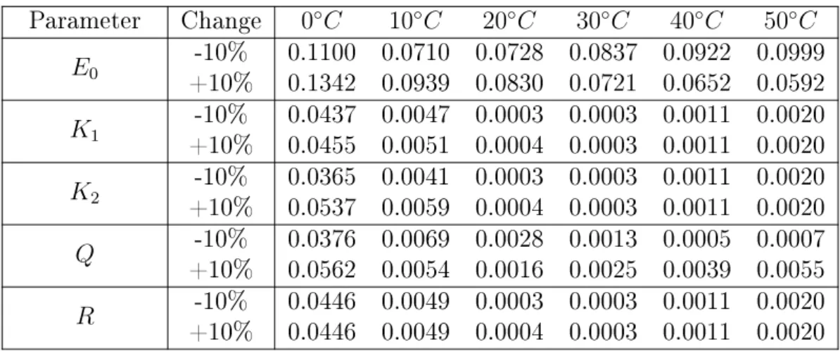
The models were simulated in Matlab using the model equations Eqs. (2.1- 2.6). At each temperatures the nominal parameters were perturbed one-by-one and the value of the loss function was computed. The result of the sensitivity analysis of the charge and the discharge model can be seen in Table 2.3 and Table 2.4. The graphical representation of the results is depicted in Figure 2.3.

Table 2.3: Values of the loss function in case of the parameter sensitivity analysis of the charge model.

Parameter Change 0^◦C 10^◦C 20^◦C 30^◦C 40^◦C 50^◦C E₀ -10% 0.1100 0.0710 0.0728 0.0837 0.0922 0.0999

+10% 0.1342 0.0939 0.0830 0.0721 0.0652 0.0592 K₁ -10% 0.0437 0.0047 0.0003 0.0003 0.0011 0.0020 +10% 0.0455 0.0051 0.0004 0.0003 0.0011 0.0020 K₂ -10% 0.0365 0.0041 0.0003 0.0003 0.0011 0.0020 +10% 0.0537 0.0059 0.0004 0.0003 0.0011 0.0020 Q -10% 0.0376 0.0069 0.0028 0.0013 0.0005 0.0007 +10% 0.0562 0.0054 0.0016 0.0025 0.0039 0.0055 R -10% 0.0446 0.0049 0.0003 0.0003 0.0011 0.0020 +10% 0.0446 0.0049 0.0004 0.0003 0.0011 0.0020

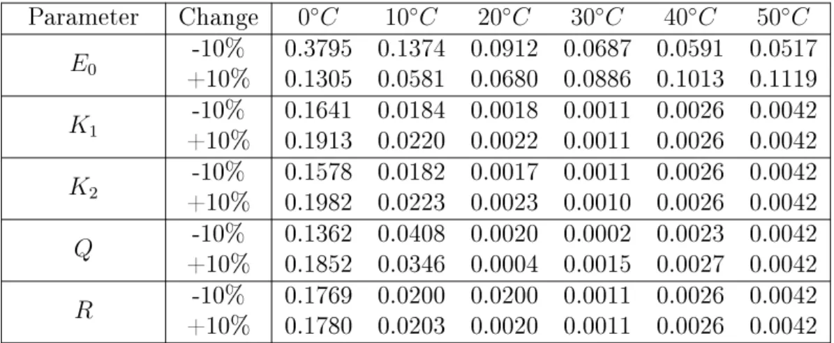
Table 2.4: Values of the loss function in case of the parameter sensitivity analysis of the discharge model.

Parameter Change 0^◦C 10^◦C 20^◦C 30^◦C 40^◦C 50^◦C E0 -10% 0.3795 0.1374 0.0912 0.0687 0.0591 0.0517

+10% 0.1305 0.0581 0.0680 0.0886 0.1013 0.1119 K₁ -10% 0.1641 0.0184 0.0018 0.0011 0.0026 0.0042 +10% 0.1913 0.0220 0.0022 0.0011 0.0026 0.0042 K₂ -10% 0.1578 0.0182 0.0017 0.0011 0.0026 0.0042 +10% 0.1982 0.0223 0.0023 0.0010 0.0026 0.0042 Q -10% 0.1362 0.0408 0.0020 0.0002 0.0023 0.0042 +10% 0.1852 0.0346 0.0004 0.0015 0.0027 0.0042 R -10% 0.1769 0.0200 0.0200 0.0011 0.0026 0.0042 +10% 0.1780 0.0203 0.0020 0.0011 0.0026 0.0042

0 20 40

0 0.1 0.2 0.3 0.4

Temperature[^◦C]

Ws(˜θ)

E₀−10% E₀+ 10% K₁−10% K₁+ 10% K₂−10%

K₂+ 10% Q−10% Q+ 10% R−10% R+ 10%

(a) Sensitivity of the charge model

0 20 40

0 0.1 0.2 0.3 0.4

Temperature [^◦C]

Ws(˜θ)

(b) Sensitivity of the discharge model Figure 2.3: Results of the parameter sensitivity analysis of the charge and the discharge model

It can be seen that the discharge model is a bit more sensitive to the change of the parameters as the magnitude of the error is greater in that case. Both the charge and the discharge models have similar characteristics with respect to the parameter sensitivity:

ˆ The models are highly sensitive to the constant potential E .

ˆ The sensitivity of the models increases as the temperature decreases.

ˆ At ambient temperatures greater than the nominal temperature, the ef- fect of changing the parameters is really small (except forE₀), especially in case of the discharge model.

ˆ The change of the internal resistance R at dierent temperatures has no eect on the models, as the errors related to the 10%change are almost the same. In these cases only the temperature aects the models.

Based on these statements the parameters E₀, K₁, K₂ and Q will be estimated while R is xed to its nominal value.

2.3.2 Input signal

The pseudo-random binary sequence (PRBS) is chosen as the input signal for the parameter estimation. It is a widely used signal in the eld of parameter estimation [60] because it is easy to generate and provides sucient excitation.

The PRBS has only two values in between the signal changes randomly. The two parameters of the PRBS are the range (the upper and lower level of the signal) and the frequency of the change that should be chosen considering the system dynamics. In our case the clock frequency of the PRBS was chosen to be 5 times the time constant of the system, the latter can be approximately determined from the step response of system (see in Section 2.3.1).

An other important factor of our parameter estimation method is the am- bient temperature. The experiments were carried out at dierent ambient temperatures that were hold constant during an experiment.

The minimum and maximum ambient temperatures of the experiments were chosen according to the recommended operating temperatures of the ex- amined battery. Then this range was evenly divided to get the list of ambient temperatures at which the experiments were carried out. For example if the operating temperature range of the battery is [0^◦C,50^◦C]then the experimen- tal ambient temperatures can be 0^◦C, 5^◦C, 10^◦C, . . . ,50^◦C.

A method for optimal design of experiments was developed in our previ- ous work [56]. In that paper two dierent input signals (CCCV (Constant Current Constant Voltage) and PRBS charge/discharge proles) were investi- gated in order to maximize the available information about the parameters to be estimated.

2.3.3 Simulation setup

The parameter estimation methods were implemented and tested by sim- ulation experiments in Matlab. To simulate the heat dissipation of the bat- tery during charge/discharge, the battery model in Simulink/Simscape/ Elec- trical/Specialized Power Systems/Electric Drives/Extra Sources (an extended model) was used[57]. This model contains additional energy balance equations that describe the temperature eects of the battery [61]. This means that the

cell temperature and the heating/cooling eects of the battery (including self- heating) during the operation can be simulated. It is important to note that the model used for parameter estimation Eq. (2.1-2.11) is much more simple, as it does not contain the internal energy balance equation. The advantage of the Simulink model is that the battery cell temperature can be directly ex- tracted from the model, which can be used as measurement data for the cell temperature.

The simulated battery was a Samsung INR18650Q-20Q battery with 2000 mAh capacity whose nominal parameters can be seen in Table 2.1 and Table 2.2. The operating temperature range of the battery from the datasheet is [0^◦C,50^◦C]for charge and[−20^◦C,75^◦C]for discharge. Based on these values, the ambient temperature was set to be between 0−50^◦C for the simulation.

The charge and the discharge of the battery was simulated at 11 dierent ambient temperatures with PRBS input signal between 1-99% state of charge.

The simulation setup in case of charge and discharge can be seen below.

Simulation setup for charge:

ˆ PRBS input: I_min =−2A, I_max =−0.5A, T_s= 160s;

ˆ initial values: q(t₀) = 0.99Q,i^∗(t₀) = 0, T =T_a;

ˆ ambient temperatures: T_a= 0,5,10,15,20,25,30,35,40,45,50^◦C;

ˆ stopping criterion: q(t) = 0. Simulation setup for discharge:

ˆ PRBS input: I_min = 0.5A, I_max = 2A, T_s = 160s;

ˆ initial values: q(t₀) = 0.01Q,i^∗(t₀) = 0, T =T_a;

ˆ ambient temperatures: T_a= 0,5,10,15,20,25,30,35,40,45,50^◦C;

ˆ stopping criterion: q(t) = 0.99Q.

All the simulations were performed on a PC (Intel i5 CPU with 4 GB RAM).

2.4 Methods for parameter estimation

The proposed parameter estimation method consists of two steps. At rst the battery is charged or discharged at dierent constant ambient tempera-

2.4.1 Estimation of the battery parameters

The rst step of the proposed method is the estimation of the battery pa- rameters at dierent constant ambient temperatures to see how these parame- ters change with the temperature. The inputs of the parameter estimation are the battery current and voltage at dierent temperatures during a full charge or discharge process. The result of the estimation is a set of battery parameters at dierent temperatures.

It can be seen from Eqs. (2.1-2.6) that the battery model has a nonlinear output equation and four parameters to be estimated. The internal resistance Rwas xed to its nominal value because the sensitivity analysis (Section 2.3.1) showed that the model is not sensitive to the parameter R. To estimate the parameters of the model a suitable nonlinear parameter estimation method should be chosen. In this work the nonlinear least-squares method was used for parameter estimation.

Nonlinear parameter estimation problems are usually solved as nonlinear optimization problems where a suitable cost function should be minimized. In our case the cost function is the sum of squared deviation between the model and the measurement data at every time instance (see Eq. (2.13) below).

W(θ) =

N

X

k=1

ˆ

v^X_b (k)−v_b^X(θ;k)2

(2.13)

X ∈ {ch;dch}

where vˆ_b^X(k) = ˆv_b^X(k T_s) is the measured value of the battery voltage at the k-th sample, v_b^X(θ;k) is the output of the model (Eq. (2.4) or Eq. (2.6)) with the parameter vector θ = [E₀, K₁, K₂, Q], and N is the total number of samples.

As all of the parameters to be estimated have physical meaning, the range and scale of the parameter values are usually known in advance. Therefore upper and lower bounds for the parameters can be dened that is useful to limit the searching space of the optimization. As a result, a constrained nonlinear optimization problem should be solved. From the potential algorithms the Trust Region Reective algorithm [62] was chosen in our work.

2.4.2 Estimation of the temperature dependency of the parameters

The second step of the parameter estimation method is the estimation of the reference values and the temperature dependency coecients of the parameters.

The inputs of this parameter estimation problem are the estimated parameters at dierent temperatures from the previous step (Section 2.4.1). It can be seen from the temperature dependent battery model, that the parameters can be divided into two groups based on the type of their temperature dependency:

ˆ Parameters with linear temperature dependency: E0, Q;

ˆ Parameters with nonlinear (exponential) temperature dependency: K₁, K₂.

Moreover it can be seen from Eqs. (2.7-2.11) that some of the parameters (Q) depend on the ambient temperature and others (E₀, K₁, K₂) depend on the battery cell temperature. The problem is that the cell temperature is not always measurable. In that case when the temperature is measured, the temperature sensor is usually placed on the surface of the battery. In addi- tion the charge/discharge current aects the heat generation of the battery, too. Charging/discharging the battery at low C rates (0.5 C - 1 C rates) we found, that the battery temperature does not increase signicantly (2^◦C). The rapid increase in the battery cell temperature can be experienced when charg- ing/disharging the battery with high C rates (5-25 C) [63]. To overcome these issues the following additional assumptions were made:

ˆ The charge/discharge current of the battery is maximum 1 C (2 A), there- fore the cell temperature does not change a lot during charge/discharge (maximum 2^◦C).

ˆ The cell temperature is substituted by the average surface temperature during charge/discharge.

ˆ Initially the cell temperature and the ambient temperature are equal (T(0) =T_a).

ˆ The surface temperature of the battery is measured.

With the above assumptions the temperature coecients of the parameters can be estimated. The coecients to be estimated are:

ˆ E₀|_Tref and ∂E/∂T for the temperature dependency of E₀;

ˆ Q|_Tref and ∆Q/∆T for the temperature dependency of Q;

ˆ K1|T_ref and α1 for the temperature dependency ofK1;

ˆ K₂|_Tref and α₂ for the temperature dependency ofK₂.

The coecients ofE₀(T)andQ(T_a)can be estimated with the simple linear least squares method because equations Eq. (2.11) and (2.10) are linear.

The coecients of K₁(T) and K₂(T) can also be estimated by the least squares method by transforming the equations and their dependent variables.

2.5 Simulation results

In this section the results of the simulation based experiments are intro-

2.5.1 Estimated battery parameters

The battery parameters at dierent temperatures were estimated using the lsqnonlin function from Matlab Optimization Toolbox [64]. This function needs at least two input arguments: a function to minimize and the vector of initial parameter values. Additional input arguments such as lower and upper bounds of the parameters and other options can be also dened. In our case the following bounds were dened for the parameters:

0 ≤ E₀ ≤ 5,

0 ≤ Q ≤ 3,

0 ≤ K₁ ≤ 0.1, 0 ≤ K₂ ≤ 0.1.

The function to minimize is the cost function in Eq. (2.13) and the parameters to be estimated are θ= [E0, Q, K1, K2]^T. The initial values of the parameters were set to the nominal parameter values (see in Table 2.1).

The results of the parameter estimation can be seen in Table 2.5 and Table 2.6. The results are also depicted in Figures 2.4 -2.7 with black dots. It can be noticed in Figure 2.5a that above 35 ^◦C (T −T_ref = 10) the battery reached its maximum capacity during charge.

Table 2.5: Estimated battery parameters at dierent temperatures during charge.

T_a[^◦C] 0 5 10 15 20 25 30 35 40 45 50

E₀[V] 3.9175 3.9154 3.9190 3.9259 3.9343 3.9436 3.9532 3.9631 3.9651 3.9783 3.9893 Q[Ah] 1.6001 1.6800 1.7599 1.8399 1.9201 2.0004 2.0811 2.1623 2.1576 2.1579 2.1582 K₁[Ω] 0.0169 0.0099 0.0059 0.0036 0.0023 0.0015 0.0010 0.0007 0.0012 0.0008 0.0007

K₂[V /Ah] 0.0246 0.0140 0.0082 0.0049 0.0030 0.0019 0.0012 0.0008 0.0000 0.0000 0.0000

Table 2.6: Estimated battery parameters at dierent temperatures during dis- charge.

T_a[^◦C] 0 5 10 15 20 25 30 35 40 45 50

E₀[V] 3.8877 3.8980 3.9083 3.9185 3.9286 3.9388 3.9490 3.9591 3.9693 3.9795 3.9884 Q[Ah] 1.6010 1.6801 1.7599 1.8393 1.9188 1.9980 2.0764 2.1540 2.2300 2.3035 2.1583 K₁[Ω] 0.0239 0.0138 0.0081 0.0048 0.0029 0.0018 0.0011 0.0007 0.0004 0.0003 0.0000

K₂[V /Ah] 0.0243 0.0139 0.0081 0.0048 0.0029 0.0018 0.0011 0.0007 0.0005 0.0003 0.0000

−20 0 20 3.9

3.92 3.94 3.96 3.98

T−Tref[K]

E0[V]

E₀(T) charge estimatedE₀

tted curve

(a) The tted thermal characteristics of parameterE₀(T)from the charge data.

−20 0 20

3.9 3.95 4

T −Tref[K]

E0[V]

E₀(T)discharge estimatedE₀

tted curve

(b) The tted thermal characteristics of parameter E₀ from the discharge data.

Figure 2.4: Estimation of the temperature dependency of E₀

−20 0 20

1.6 1.8 2 2.2 2.4

Ta−Tref[K]

Q[Ah]

Q(Ta) charge estimatedQ

tted curve

(a) The tted thermal characteristics of parameterQ from the charge data.

−20 0 20

1.6 1.8 2 2.2 2.4

Ta−Tref[K]

Q[Ah]

Q(Ta) discharge estimated Q

tted curve

(b) The tted thermal characteristics of parameter Qfrom the discharge data.

Figure 2.5: Estimation of the temperature dependency of Q

−2 0 2

·10⁻⁴ 0

0.5 1 1.5

·10⁻²

1 T −_T¹

ref

₁

K

K1[Ω]

K₁(T) charge estimated K₁

tted curve

(a) The tted thermal characteristics of parameter K1(T) from the charge data.

−2 0 2

·10⁻⁴ 0

1 2

·10⁻²

1 T −_T¹

ref

₁

K

K1[Ω]

K₁(T) discharge estimatedK₁

tted curve

(b) The tted thermal characteristics of parameter K₁(T) from the discharge data.

Figure 2.6: Estimation of the temperature dependency of K₁

−2 0 2

·10⁻⁴ 0

1 2 3

·10⁻²

1 T −_T¹

ref

₁

K

K2[V/Ah]

K₂(T)charge estimatedK₂

tted curve

(a) The tted thermal characteristics of parameter K2(T) from the charge data.

−2 0 2

·10⁻⁴ 0

1 2

·10⁻²

1 T −_T¹

ref

₁

K

K2[V/Ah]

K₂(T) discharge estimatedK₂

tted curve

(b) The tted thermal characteristics of parameter K2(T) from the discharge data.

Figure 2.7: Estimation of the temperature dependency of K₂

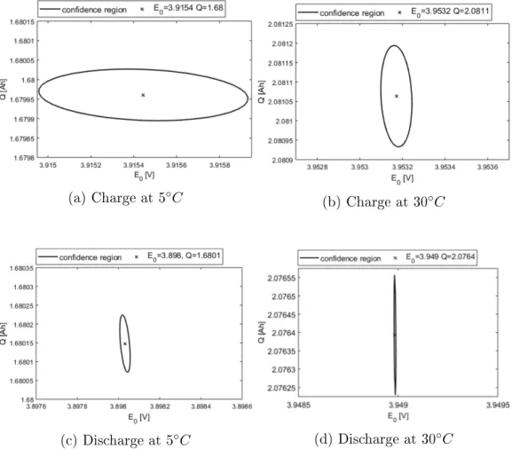
It can be seen from the estimated values that they are in good agree- ment with the nominal parameters of the investigated battery type, and co- incide well with the parameters in the detailed dynamic battery model in Simulink/Simscape/Electrical/Specialized Power Systems/Electric Drives/Extra Sources.

The accuracy of the parameter estimation can be characterized by the co- variance matrix of the estimation. In our results the elements of the covariance matrices are really small (with orders between10⁻⁸ and 10⁻¹²) in both charge and discharge cases. This means that the parameter estimation is very accu-