73
Zoltán Szántó–István György Tóth
DOUBLE OR QUITS: SHOULD MONEY FOUND BE RISKED?
An attempt to measure attitudes towards risk using survey methods
1This article examines social attitudes towards risk-preference and risk-aversion.
First, we briefly discuss the theoretical approach to the analysis of risk-preference and risk-aversion that was developed within rational choice theory. Next, we present an approach to operationalise risk-preference using survey data. Our measurement of attitudes towards risk follows the usual strategy: respondents are asked to choose between a small amount of money they get for sure, and a large but risky amount.
Drawing on the theoretical models and earlier empirical research, we formulate hypotheses about the social factors that have an impact on actual decision making in the situations under study. The hypotheses are tested using survey data. The article ends with a brief discussion. The novelty of our paper is that – to the best of our knowledge – neither previous Hungarian nor international research has attempted to examine attitudes towards risk using data from large-scale surveys.
The analysis of attitudes towards risk Certainty, uncertainty, and risk
Rational choice theory makes a distinction between perfect and imperfect information about the states of the world that are relevant in decision making situations, and thereby about the outcomes that will follow from alternative courses of action (Elster 1986: 5). When, for example, a farmer must choose between two grain varieties he or she should bear in mind that the size of the crop next year will depend on future weather conditions, which, however, cannot be predicted with
1 This article is a revised version of a paper that was presented at the workshop Action Theory and Social Research [Cselekvéselmélet és társadalomkutatás] (27–28 November 1998, Budapest), which was dedicated to the memory of László Csontos. Both authors are indebted to Csontos, who taught us both professional and human values. The basic questions of this paper goes back to the idea he developed with one of the authors to examine the relationship between attitudes towards risk and attitudes towards the reform of welfare systems, as a follow-up to the research project The state and its citizens [Az állam és polgárai] (Csontos–Kornai–Tóth 1996; Csontos–Tóth 1998). The survey questions analysed in our paper were suggested by László Csontos. Our work was financially supported by the National Science and Research Foundation (OTKA) (research grant F 022195).
Comments and suggestions are welcome. Please direct correspondence to:
zoltan.szanto@soc.bke.hu and toth@tarki.hu. We are grateful to Róbert Iván Gál for his helpful comments on an earlier version of this paper, and to Tamás Bartus for the translation of this article.
certainty. Virtually all actual situations are of this kind but some of them approximate very closely the extreme case of certainty. We have certainty when decision-makers know which of the possible states of the world will occur, and thereby which of the possible consequences will ensue: one of the states of the world occurs with probability one, and the other states of the world occur with probability zero.
Consider our farmer who must choose between two grain varieties, A and B (Elster 1995: 34–35; 1986: 6). There are two possible weather conditions (states of the world), good and bad. Using available information, our farmer assumes that both conditions have an equal probability of occurring (50–50 per cent). The income of the farmer and the utility of the respective incomes in the various cases are shown in Table 1. Utilities reflect the decreasing marginal utility of money: the utility of one additional dollar falls with the number of dollars.
Table 1. Outcomes in situations involving risk
Grain A Grain B
Weather income
(in US dollar)
utility (U)
income (in US dollar)
utility (U)
Good 30,000 47 50,000 50
Bad 25,000 42 15,000 33
Average 27,500 45 32,500 48
Choice situations where available information is incomplete may be characterised by risk or by certainty. Broadly speaking, we have certainty when actors know which of the states of the world can occur. Risk refers to situations where actors are able to attach – either objective or subjective – probabilities to the states of the world.
Uncertainty refers to situations where actors do not know these probabilities.
There is considerable disagreement between classical and Bayesian decision theories about whether or not all situations of uncertainty can be represented in terms of risk. Recent developments point towards the acceptance of the Bayesian view. As Bayesian scholars argue (Hirshleifer–Riley 1992: 9–11), rational actors are always able to assign – to some extent reliable – probabilities to the states of the world on the basis of available information. Additionally, all probabilities are subjective. The distinction between uncertainty and risk disappears: rational decision-makers should choose the act which maximises the (subjective) expected utility. The expected utility of an act is the weighted sum of the utilities of the consequences, where the weights are the probabilities with which the consequences occur.
Risk-aversion, risk-neutrality, risk-preference
To analyse attitudes towards risk, let us consider Table 1 again. Clearly, crop B has the highest expected yield. It need not, however, have the highest expected utility and hence need not be the one which a rational agent would choose. If an income of
$20,000 is required for subsistence, our farmer would be foolish to prefer a course of action that gave him a 50 per cent chance of starving to death. This is a special case of the more general fact that money has a decreasing marginal utility, which implies
that the utility of expected income is larger than the expected utility of income (Elster 1986; Varian 1991). In our example,
U[(50 000/2+15 000)/2]>[U(50 000)+U(15 000)]/2 = 48>41.5.
Rationality dictates the choice of the act with the largest expected utility, and this need not be the option with the largest expected income – even when all utility is derived from income. This phenomenon is referred to as risk-aversion.2
To generalsze this example, consider the following situation (Hirshleifer–Riley 1992: 16–19; Morrow 1994: 36–37). A decision-maker can choose between A and B.
If A is chosen then he or she receives the intermediate outcome C for sure. If B is chosen then he or she gets the best outcome H with probability p or the worst outcome L with probability (1–p). To be more concrete, imagine the following scenario. Option A is receiving 1000 dollars for sure. Option B is receiving 2000 dollars with probability p and receiving nothing with probability (1–p). Clearly, the choice between A and B depends on the value of p. If it is close to 1 then B will be chosen, and if p is close to zero then A will be chosen. Between the two extremes there must be a value p* where the decision-maker is indifferent between A and B. It can be proven that p* is the cardinal utility of outcome C3: U(C) = p*. Imagine that our decision-maker is indifferent between A and B if p*=3/4. This decision-maker is said to be risk-averse. A person is risk-averse if he or she strictly prefers a certain consequence to any risky prospect whose mathematical expectation of consequences equals that certainty. If his or her preferences go the other way he or she is a risk- preferrer. And if he or she is indifferent between the certain consequence and the risky prospect he or she is risk-neutral (Hirshleifer–Riley 1992: 23).
Figure 1 displays three elementary utility functions: Ura would apply to a risk- averse individual, Urn to someone who is risk-neutral, and Urp to a risk-preferrer.
Consequences and their utilities are on the vertical and horizontal axes, respectively.
The risk-averse, the risk-neutral and the risk-preferrer individuals attach the same utilities to the worst and to the best outcomes. In our example, the risk-neutral person is indifferent between A and B if p*=1/2. For risk-neutral persons the utility function, Urn is linear because the expected utility of consequences equals the utility of expected consequences. The risk-averse person is indifferent between A and B if 1/2<p*<1 depending on the extent to which he or she avoids risk. In case of risk- aversion, the elementary utility function, Ura is concave because the expected utility of consequences is less than the utility of expected consequences. The risk-preferrer
2 Here, risk-aversion is assumed to be a consequence of decreasing marginal utility. It could also, however, derive from a cautious, conservative attitude towards risk-preference (Elster 1986: 29; note 16.).
3 It is important to realise that the argument assumes the preference-scaling (or elementary utility) function defined over consequences, and not the utility function defined over actions.
Neglecting this distinction leads to misunderstandings and fruitless debates (see Hirshleifer–
Riley 1992: 13–15; 19). Note that the preference-scaling function assumes a cardinal scale, while the utility function defined over alternatives assumes only an ordinal scale. The requirement that the preference-scaling function must be cardinal is a necessary condition for the applicability of the expected utility rule. The usual method to establish such a cardinal scale is the reference-lottery technique (ibid. 16.).
individual is indifferent between A and B if 0<p*<1/2 depending on the extent to which he or she likes risks. For risk-preference the elementary utility function, Urp is convex because the expected utility of consequences is larger than the utility of expected consequences.4
Figure 1.
Preference-scaling functions for risk-aversion, risk-neutrality, and risk-preference5
U(H)=1 Ura(C)=3/4
Urn(C)=1/2
Urp(C)=1/4
Ukker(LR)=0
L C H
0 1000 2000
Consequence
Utility
The empirical model of attitudes towards risk General framework
Our study tries to identify the determinants of attitudes towards risk. The main research question is which social, demographic, and other factors have an impact on risk-preference. Our model postulates that attitudes towards risk depend on the size
4 Mathematically, the first derivatives of these three utility functions are positive: the function is rising, the marginal utility of consequences is positive. This means that more income is preferred to less. The second derivative of the preference function is zero for the risk-neutral case, it is negative for risk-averse people, and it is positive for risk-preferrer individuals. In other words, the function increases at a constant, decreasing, and increasing rate, respectively. Among the three cases, risk-aversion is considered to be the normal case because only it reflects the principle of decreasing marginal utility. Another justification is that people typically hold diversified portfolios (Hirshleifer–Riley 1992: 25).
5 The standard model we presented assumes that individual preferences and decisions are independent of the endowment of decision-makers. For relaxing this assumption, and for the constructive criticism of the expected utility rule, see the famous prospect theory (Kahneman and Tversky 1979, 1981), and the review presented in Thaler (1987). See also Csontos (1995) and Thaler and Johnson (1990).
of the expected gain/loss, on the one hand, and on the income, occupation, education, age, and gender of the respondent, on the other hand:
ATR = f(VGL, INC, OCC, EDU, AGE, SEX), where
ATR: attitudes toward risk, VGL: value of gains/losses, INC: income of the respondents,
OCC: occupation/labour-market status of respondents, EDU: educational level of respondents.
The empirical analyses are based on the assumption that among these variables only income and the value of gains/losses are perceived as decision parameters since gains and losses modify income. In contrast, variables like occupation, education, age, and sex are assumed to be factors which have an impact on preferences.
Data and methods
Measurement. The measurement of attitudes towards risk follows the common strategy of previous research. Respondents are asked to choose between two options:
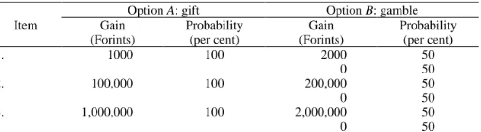
between a „gift” they receive for sure and a gamble which yields twice as much as the gift with a probability of 50 per cent, and yields nothing with a probability of 50 per cent. Three questions were repeated after each other. The questions were the same with the important exception that the amount of the gift was raised. The structure of the questions is summarised in Table 2.
Table 2. The structure of survey questions
Option A: gift Option B: gamble
Item Gain
(Forints)
Probability (per cent)
Gain (Forints)
Probability (per cent)
1. 1000 100 2000
0
50 50
2. 100,000 100 200,000
0
50 50
3. 1,000,000 100 2,000,000
0
50 50
Data. Data come from two surveys of the Social Research Centre (TÁRKI), which were held in October 1996 and January 1997, respectively. The questions described above were included in the questionnaire in both surveys. The wording of the questions was identical. Both surveys represent the population above 18 years of age. A stratified multi-stage probability sampling design was used, and registered interviewers conducted the interviews. The sample size is 1,500 in both surveys.
Since the samples were representative of the Hungarian adult population along the most important social and demographic dimensions, weighting was not necessary.
Because of the similarities of the surveys – they contained the same key questions with identical wording, they were close to each other in time, and they both
represent the Hungarian adult population –, we decided to merge the two data sets.
Pooling them was necessary to increase the sample size and thereby to enable more refined analyses. The subsequent analyses will use 3,000 cases. We can be 95 per cent confident that the results from our sample deviate only by around 1.5–2 per cent from the value we would have obtained had we included the whole population in the survey.
Interview context. The questions about risk-preference were first embedded in a block of questions about the reform of the pension system, and second in an ISSP6 module about attitudes towards the role of government and attitudes towards work.
At the end of each survey, there was a detailed module about politics. Our questions, however, were always followed by biographical information, mostly about the respondents’ labour-market position, and by questions about the respondents' knowledge about and attitudes towards the reform of the pension system.
Hypotheses
Before we formulate concrete hypotheses, we turn again to our analytical model.
The dependent variable in the model is attitudes towards risk. First, we must measure risk-aversion, risk-neutrality, and risk-preference. The survey question was worded as follows: „Would you choose the sure gain or the gamble?” Following the expected utility paradigm, the expected values of both options are considered as equal: the expected values are 1000, 100,000,and 1,000,000 Forints in each round, respectively. In this case, if the respondents had been offered the option of indifference those who are risk-neutral might have chosen this option. This alternative, however, was not included. Hypotheses can be developed for the extent to which the population of people choosing either option differs. If the respondents were indifferent but were forced to make a choice, half of them would choose the gift and half of them would choose the larger but uncertain gain. However, the standard literature about decision-making suggests that in such situations risk- aversion is the typical attitude. Keeping expected value constant, risk-averse individuals prefer sure gifts to gambles, which is consistent with the definition of risk-aversion given above. Thus, our first hypothesis is:
Hypothesis 1. (H1.): In decision situations involving risky gains, risk-aversion is the typical attitude towards risk.
This hypothesis is supported if the number of people choosing the gift is significantly larger than the number of people choosing the gamble. The hypothesis clearly follows from the theoretical model and it is supported by a vast number of empirical studies that were mainly carried out in experimental settings.7
Modelling the decision situation can be refined if we attribute the following reasoning to the respondents: „Giving an answer to the question means having one
6 International Social Survey Programme. Since 1985, when the program started, TÁRKI is the official partner of the program. The survey questions analysed here were not included in the ISSP module.
7 The experimental results of Kahneman and Tversky clearly support the hypothesis that risk- aversion is common when outcomes are gains. See for example Kahneman and Tversky 1981.
thousand Forints. If I risk this amount I either win twice as much or I loose what I had.” What is interesting in this reasoning is not that it shows that people are risk- averse, but that it shows that there are people who would risk – on a double or quits basis – a sure gift. Thus, hypothesis 1 is not exclusive. Although risk-aversion is typical for gains, there are decision-makers who display risk-preference.8 This insight can be considered an extension to hypothesis 1.
Hypothesis 1a (H1.a): In decision-making situations involving risks, we can find risk-preference along with risk-aversion.
This extension claims only that there are people who display risk-preference. The extension has a theoretical significance: it makes explicit that different attitudes towards risk exist at the same time, thus it is possible to resolve the standard assumption of economics that actors have identical preferences (utility functions).9
In the following, we examine the factors which determine the attitudes specified in hypotheses 1 and 1a. We start with the most apparent factor, the size of the gain.
In the decision situations under study, we have two outcomes: the sure gift (1000) and the risky prize (2000). Correspondingly, we can move along two dimensions.
On the one hand, assuming that the risk-free gift, is fixed, increases in the prize should increase risk-preference. On the other hand, when taking the risky outcome fixed, we may assume that increases in risk-free gift are likely to reduce risk- preference.
Given the survey questions, a hypothesis can be formulated which takes both the sure and the risky outcomes simultaneously into account. The frequency of risk- preference will depend on the expected values of gambles:
Hypothesis 2. (H2.): the higher the expected values of the options, the smaller the likelihood of displaying risk-preference.
The reasons are the same as in case of hypothesis 1a: the larger the risk-free gift, the lower the willingness to incur a risk. This effect is expected to be stronger than the effect of the increases in the value of the gain.
Next, we formulate hypotheses about the relationship between socio-economic characteristics and attitudes towards risk. Obviously, the income of the respondent is expected to play a special role. Including income as an independent variable is motivated by the principle of decreasing marginal utility of money. To put it simply, one additional dollar has a relatively small utility for those who have a relatively large income. This would be especially the case if the costs of producing the income were also taken into account. If the assumption of the decreasing marginal utility of money is correct then we have the following hypothesis:
Hypothesis 3 (H3.): Keeping other factors constant, risk-preference increases with income.
8 According to prospect theory, risk-preference is the typical attitudes when outcomes are losses. We do not formulate hypotheses about losses since our study is restricted to gains.
9 The programmatic statement can be found in Becker and Stigler (1977). Later, Becker (1996) argued that utility functions are the same for different people, and they are stable over time. For a criticism, see Elster (1995): „Most social scientists, however, believe that people differ in their desires as well as in their opportunities […]” (p. 15.)
This hypothesis says only that if a person’s income increases then the value of the lost gift becomes less significant when choosing the gamble.10
We have intuitive rather than well-founded reasons for the assumed impacts of socio-economic characteristics that are expected to have on attitudes towards risk.
We formulated three additional hypotheses. We believe that the factors specified in the hypotheses have an indirect effect on attitudes towards money, spending, and risk directly and by composition effects as well.
Hypothesis 4 (H4.): the likelihood of displaying risk-preference increases with education.
Hypothesis 5 (H5.): the likelihood of displaying risk-preference decreases with age.
Hypothesis 6 (H6.): men are more likely to display risk-preference than women.11 Later we will argue that experimental situations like this often produce sterile results. Using available data, it is worthwhile to examine the empirical relationship between attitudes towards risk, as defined in an experimental situation, and actual behavior, like having insurance or having savings as preparation for old age.
Occupation is very likely to be one of the factors that determine risk-preference. The following hypothesis seems to be plausible:
Hypothesis 7 (H7.): Occupational status has a direct impact on risk-preference, which cannot be attributed to compositional factors. More precisely, we believe that occupation has an aspect which is independent of other attributes, like education, sex, age, and income. This aspect may be attributed to freedom of command and autonomy when practicing a job.
Analyses
Risk-preference: descriptive statistics
We begin our analyses by examining the proportion of people who have chosen the gamble at different levels of gains/losses. The results are shown in Table 3.
10 Previous research produced other hypotheses. For example, Hirshleifer and Riley (1992:
26–28.) claim that risk-aversion is typical among the poor and the rich, and risk-preference is the typical attitude for people having an intermediate income. This claim contradicts our hypotheses and intuition. In the following, we restrict the analyses to our more plausible hypothesis, which is consistent with the assumption of the decreasing marginal utility of money.
11 Previous research found that young men very often display risk-preference (cf. Hirshleifer and Riley 1992: 28). Our hypotheses H5. and H6. are consistent with these findings.
Table 3. Proportion of respondents choosing the gamble as a percentage of all respondents
Sample
Gain (in HUF) 1996 1997 Pooled data
Small (1,000) 36.3 31.6 34.0
Intermediate (100,000) 18.3 16.4 17.4
Large (1,000,000) 7.8 7.4 7.6
Comparing the two samples reveals that the results from the two samples are very similar. There is no significant difference in the proportion of people choosing either gamble between the two samples (note that for a sample size of 1500 the sampling error is around 2.5–3 per cent).12
This is not the only result. The gamble is chosen by 34, 17, and 7.6 per cent of the respondents if the prize is small, intermediate, and large, respectively. It is easy to see that the number of people choosing the gamble is about one-third of the population even when the prize is the smallest. The fact that more than the half of the respondents avoid any risk shows in an indirect way that people are rather risk- averse (see hypothesis 1). Nevertheless, one in 12-13 people would risk even the highest price for the gamble (see hypothesis 1a).
We can go further if we examine the decisions individuals made in each subsequent round. Table 4 displays the proportion of people choosing either the gift or the gamble for each level of gain. The cells contain the distribution of people choosing these options. Bold numbers and numbers in italics are the proportion of those who have chosen the gamble and the gift, respectively. The next cell shows the same distribution in the next round. For example, the number in the upper left cell indicates that 66.2 per cent of respondents have chosen the risk-free gift in the first round. After rising the prize, 97.5 per cent keeps choosing the gift, and only 1.1 per cent chooses the gamble in the last round.
The inspection of data leads to the following conclusions. People who have chosen the gift in the first round keep choosing it in subsequent rounds as well.
Those people, however, who undertook a risk in the first round, were less likely to incur a risk in the subsequent rounds. Among those who choose the gamble in the first round, 54 per cent chooses the gift in the second round, and 97 per cent choose it in the last round.
12 This analysis is important because it supports indirectly our decision to stack the samples.
The samples are similar not only with respect to the most important socio-economic factors but also with respect to the distribution of the dependent variable.
Table 4. The probability of choosing the gamble conditional on choosing or rejecting the gamble in the previous round: the distribution of respondents choosing the gamble (number in italics) and of those choosing the gift (bold number) Small gain
(1,000 HUF)
Intermediate gain (100,000 HUF)
Large gain (1,000,000 HUF)
98.9 97.5
66.2 1.1
66.0 2.5
34.0 97.1 54.1
2.9
33.8 64.0
45.9
36.0
These results support hypothesis 2. There is a clear tendency towards a decrease in the proportion of people choosing the gamble as the size of the gain increases.
A simple bivariate analysis of the data revealed a J-shaped relationship between income and risk-preference.13 Risk-preference relatively often occurs in the low- income regions, then it becomes less frequent, and finally, it increases in high- income regions. We also found that the effect of income on risk-preference is smaller for high prizes than for small prizes (these results refine rather than fully support hypothesis 3.) Risk-preference decreases with age, as expected on the basis of hypothesis 5, but it increases with education (hypothesis 4). More precisely, risk- preference occurs less often among people with primary education than among people with secondary or higher education. Finally, men are more likely to display risk-preference than women (hypothesis 6).
It can, however, be the case that these results are due to compositional effects.
For example, the difference in risk-preference between men and women might be explained in terms of differences in income, education and age rather than in terms of differences in socialization or „genetics”. Similarly, differences between educational levels might disappear if we control for other variables. Therefore, we examine which of the variables specified earlier have a significant effect on risk- preference with a multivariate technique.
Logistic regression is appropriate for this purpose. Logistic regression applies to situations where the dependent variable is binary (dummy variable), while the independent variables may be categorical, ordinal or interval. Furthermore, contrary to other methods, it does not require that strong assumptions about the distribution of variables. Logistic regression predicts the probability of occurrence of certain events. In case of many variables, the probability of events is modelled using the following equation:
13 These analyses are not reported in detail here.
Prob(event)=1/(1+e–Z), where
e is the basis of natural logarithm, approximately 2.718,
Z is the linear combination of variables and parameters. Z can be written as Z=B0+B1X1+B2X2+ ... BkXk,
where
X1, X2, ... Xk are the explanatory variables, B0 is the constant, and B1, ... Bk are the respective parameters.
In our model, the dependent variable is the attitude towards risk, measured as choosing the gamble in each round (GAMBLE1, GAMBLE2 and GAMBLE3, choosing the gamble = 1, choosing the sure gift = 0).
The independent variables are defined as follows:
LG10INC = 10 base logarithm of household income (we use the log transformation because incomes are log-normally distributed and the logarithmic specification is expected to yield higher explanatory power).
AGE = age of the respondents grouped into 6 cohorts (–29, 30–39, 40–49, 50–59, 60–69 and 70-),
EDUi= highest educational level of respondents (i = 1: primary education or less, i = 2: secondary education, and i = 3: tertiary education),
SEX = sex of the respondents (0= female, 1= male),
SELFEMP = employment status of respondents (1=self-employed, 0= otherwise) We estimated three models that reflect choices in the three rounds. The first model contains only these variables. Modelling the second and the third round also takes into account whether the respondents choose the gamble in the previous round(s).
Thus, our models are as follows:
prob(GAMBLEi) = 1/(1+e–Z), where
Z=B0+B1*LG10INC+B2*AGE+B3*EDU+B4*SEX+B5*SELFEMP.
Estimation results for these three models are summarised in Table 5. All independent variables were entered simultaneously (METHOD=ENTER). The second column shows the parameter estimates. The columns Wald and Significance display the Wald-statistics and the respective significance levels. These columns tell us the level at which we can be confident that the observed difference of parameters from zero is a result of chance only. Bold numbers and numbers in italics are the variables which have a significant effect at p<0.05 and p<0.1 levels, respectively.
Numbers not marked in either way are the coefficients which do not represent significant effects at these levels. The reason behind finding no significant effects is either the absence of any causal effect or the fact that there is an effect, but it is
suppressed or not linear. The last column of the table displays odds ratios. Odds ratios indicate how much the odds of the dependent variable increases if the value of the independent variable under study increases by one unit.
In the first round (GAMBLE1), income (LG10INC) and education (EDU) have a positive and significant effect on risk-preference. The effect of AGE is significant at this level, as well, but its overall effect is negative. The effect of sex is substantially weaker, and employment status (SELFEMP) has no effect at all. The income variable has an odds ratio of 2.4, which means that the odds of choosing the gamble increases by a factor of 2.4 if the logarithm of income increases by 1 unit (or income itself increases by a factor of 10). Imagine a person whose income is 100 thousands Forints. Keeping all other factors constant, if the probability of the gamble is 30 per cent for an income of 10 thousands Forints (the corresponding odds is 3/7 = 0.42), our person chooses the gamble with an estimated probability of 50-51 per cent (the corresponding odds is 3×2.4/7 = 1.03).
In the second round (GAMBLE2), all independent variables have a significant effect at the p<0.05 level except education and sex which are significant only at p<0.1 level. The effect of AGE is substantially weaker than it was in the first round.
The variables which have stronger effects on risk-preference are employment status (SELFEMP) and choosing the gamble in the first round.
Table 5. Logistic regressions of choosing the gamble in each round: all independent variables entered simultaneously
Variable Coefficient Standard error
Wald Significance R Odds ratio:
exp(B) Gain: 1000 Forints (GAMBLE1)
LG10INC 0.8897 0.2261 15.4899 0.0001 0.0684 2.4344
AGE –0.2397 0.0311 59.5491 0.0000 –0.1412 0.7869
EDU 0.2404 0.0802 8.9806 0.0027 0.0492 1.2718
SEX 0.1645 0.0929 3.1380 0.0765 0.0199 1.1788
SELFEMP -0.1335 0.1972 0.4580 0.4985 0.0000 0.8751
Constant -4.6227 1.0125 20.8463 0,0000
Gain: 100,000 Forints (GAMBLE2)
LG10INC 0.8088 0.3315 5.9522 0.0147 0.0442 2.2453
AGE –0.0936 0.0473 3.9211 0.0477 –0.0308 0.9106
EDU 0.2378 0.1236 3.7044 0.0543 0.0290 1.2685
SEX 0.2491 0.1385 3.2362 0.0720 0.0247 1.2829
SELFEMP 0.7679 0.2777 7.6453 0.0057 0.0528 2.1553 GAMBLE1 3.3653 0.1815 343.929
9
0.0000 0.4112 28.9410
Constant –7.7045 1.5014 26.3312 0.0000
Gain: 1,000,000 Forints (GAMBLE3)
LG10INC –0.8691 0.4258 4.1658 0.0412 –0.0435 0.4193
AGE 0.0727 0.0660 1.2121 0.2709 0.0000 1.0754
EDU 0.0457 0.1726 0.0702 0.7910 0.0000 1.0468
SEX -0.0698 0.1916 0.1329 0.7154 0.0000 0.9325
SELFEMP 0.0524 0.3545 0.0218 0.8825 0.0000 1.0538
GAMBLE1 0.3305 0.2863 1.3327 0.2483 0.0000 1.3917
GAMBLE2 3.4064 0.2882 139.683 8
0.0000 0.3468 30.1563
Constant –0.5330 1.9001 0.0787 0.7791
When the prize is the highest (GAMBLE3), there are only two variables which have a significant effect on risk-preference: household income (LG10INC) and, more importantly, choosing the gamble in the second round (GAMBLE2). Note that the coefficient of income (LG10INC) is negative, which means that keeping other factors constant, a rise in income decreases the likelihood of displaying risk- preference.
The regressions were also run using the backstep procedure. This means that after entering all independent variables, we removed the variables which were not significant, and we re-estimated the models using only the significant variables. The resulting models include only variables with actual explanatory power. The results are displayed in Table 6.
Table 6. Logistic regressions of choosing the gamble in each round using the backstep procedure
Gain (in HUF)
Variable 1000
(GAMBLE1)
100,000 (GAMBLE2)
1,000,000 (GAMBLE3)
Constant -4.5669 -7.7045 -0.1523
Lg10JOV 0.8762 0.8088 -0.869
AGE -0.2391 -0.0936 n.s.
EDU 0.2398 0.2378 n.s.
SEX 0.1600 0.2491 n.s.
SELFEMP n.s. 0.7679 n.s.
GAMBLE1 3.3653 n.s.
GAMBLE2 3.5797
Degrees of freedom 4 6 2
Model χ2 144.672 693.180 362.276
Significance 0.0000 0.0000 0.0000
per cent of correct classification 68.59 85.95 93.2
Using the coefficients in Table 6, we can predict the probability of displaying risk- preference as a function of the significant variables. Consider, for example, a male respondent (SEX = 1) aged 29 (AGE = 1) who has a university education (EDU3 = 3) and who lives in a household where the household income is 40 thousands Forints per person. The probability that he chooses the gamble in the first round can be calculated as follows:
Since lg10 (40 000)=4.61,
Z = –4.5669+0.8762×4.61-0.2391×1+0.2398×3+0.1600×1=0.1127, and hence, prob(GAMBLE1)=1/(1+2.718–0.1127) = 0.5281,
thus our respondent with the above defined characteristics chooses the gamble with an estimated probability of 53 per cent.
Consider now a women (SEX = 0) aged above 70 (AGE = 6) who has only elementary education (EDU = 1) and who lives in a family where household income is 15 thousands Forints per person. Her probability of choosing the gamble in the first round is given by
prob(GAMBLE1)=1/(1+2.718–(–2.099))=0.1092 where
Z = –4.5669+0.8762×4.18-0.2391×6+0.2398×1+0.1600×0 = –2.099, and the number 4.18 = lg10 (15 000)
In short, she will choose the gamble with an estimated probability of around 11 per cent.
To develop a more general and transparent interpretation of the results, we set the significant explanatory variables to certain values and we calculate the probability of displaying risk-preference for the defined values. The values we chose reflect typical demographic and social situations. Our aim here is to show how the probability of choosing the gamble varies with income for each socio-economic type.
For the first round (model GAMBLE1), the following types are defined:
1. male below 29 years of age with tertiary education (type 1), 2. female aged 40–59 with secondary education (type 2), 3. female over 70 with primary education (type 3).
The risk-preference functions calculated for these typical cases are displayed in Figure 2. The functions are calculated separately for the three rounds. First, consider the model GAMBLE1. The probability of displaying risk-preference increases with income for each typical case. It is the 29 years old male who is most likely to display risk-preference. This probability is the lowest if the 70 years old woman is considered. Note that risk-preference rises with income somewhat steeper for the later case than for the former one if income is high.
Figure 2.
The probability of choosing the gamble with expected value 1000 Forints as a function of income, for typical combinations of social-economic characteristics
prob(type 1) prob(type 2) prob(type 3)
0,0 0,1 0,2 0,3 0,4 0,5 0,6 0,7 0,8 0,9 1,0
20000
0 500000
The probability of choosing the gamble
Income, log scale
For the model GAMBLE2, where the expected value is 100 thousands Forints, the typical cases are as follows:
1. male below 29 years of age with tertiary education who is self-employed and who chose the risky option in GAMBLE1 (type 1),
2. female aged 40–49 with secondary education who is employee and who chose the risky option in GAMBLE1 (type 2),
3. male aged 40–49 with secondary education who is employee and who chose the risky option in GAMBLE1 (type 3),
4. female over 70 years old with primary education who is employee and who chose the risky option in GAMBLE1 (type 4),
The income–GAMBLE2 function is displayed in Figure 3.
Figure 3.
The probability of choosing the gamble with expected value 100,000 Forints as a function of income for typical combinations of social-economic characteristics
0,0 0,1 0,2 0,3 0,4 0,5 0,6 0,7 0,8 0,9 1,0
prob(type 1) prob(type 2) prob(type 3) prob(type 4)
Income, log scale
0 20000 500000
The probability choosing the gamble
The dispersion of probabilities of risk-preference is larger than that was in GAMBLE1. This is not surprising since the explanatory power of each variable is higher than in the first round. Again, we find that the probability of risk-preference increases more steeply with high gains among those who are unlikely to take a risk if the prize is low than among those who are likely to incur a risk already in the first round.
Finally, two typical cases were defined to interpret model GAMBLE3 (expected value was 1 million Forints):
1. a person who chose the risky gamble neither in the first nor in the second round;
2. a person who chose the risky gamble both in the first and in the second round.
The income-GAMBLE3 functions are displayed in Figure 4. The falling shape of the curves reflects the negative sign of the income variable in the third round. The figure clearly shows that those who chose the gamble in the first two rounds are likely to choose the third gamble too. This means that if the prize is large, like 1 million Forints, only those are likely to incur a risk who have relatively small income and who are fond of gambling anyway (choosing the gamble in the previous rounds).
Figure 4.
The probability of choosing the gamble with expected value 1,000,000 Forints as a function of income depending on participation in earlier gambling
prob(j0;j0) prob(j1;j1) The probability of
choosing of gamble
0,0 0,1 0,2 0,3 0,4 0,5 0,6 0,7
0 20000 500000
Income, log scale
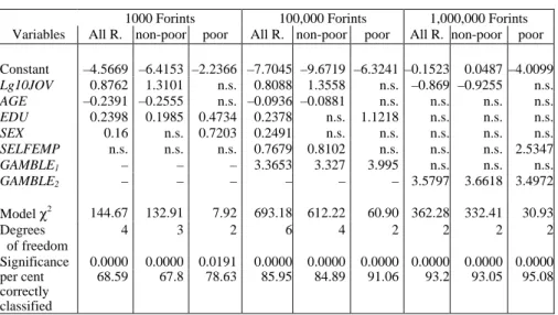
Examining non-linear relationships. Earlier in this paper when we examined hypothesis 3, we found a J-shaped relationship between income and the probability of choosing the gamble. Since logistic regression assumes a linear relationship between the probability of the event and the independent variables, we must cope with this problem. The bivariate analyses showed that the cutoff point for the J- shaped relationship is close to half of the median income. Below and above this point the relationships seem to be linear. Correspondingly, we can examine the relationship between risk-preference and income separately in two groups: among those who have less, and those who have more income than half the median. The results are summarised in Table 7.
Table 7. Logistic regressions predicting choice of gamble in each round using the backstep procedure; models estimated separately for the poor, for the non-poor, and for all respondents.
1000 Forints 100,000 Forints 1,000,000 Forints Variables All R. non-poor poor All R. non-poor poor All R. non-poor poor Constant –4.5669 –6.4153 –2.2366 –7.7045 –9.6719 –6.3241 –0.1523 0.0487 –4.0099 Lg10JOV 0.8762 1.3101 n.s. 0.8088 1.3558 n.s. –0.869 –0.9255 n.s.
AGE –0.2391 –0.2555 n.s. –0.0936 –0.0881 n.s. n.s. n.s. n.s.
EDU 0.2398 0.1985 0.4734 0.2378 n.s. 1.1218 n.s. n.s. n.s.
SEX 0.16 n.s. 0.7203 0.2491 n.s. n.s. n.s. n.s. n.s.
SELFEMP n.s. n.s. n.s. 0.7679 0.8102 n.s. n.s. n.s. 2.5347 GAMBLE1 – – – 3.3653 3.327 3.995 n.s. n.s. n.s.
GAMBLE2 – – – – – – 3.5797 3.6618 3.4972 Model χ2 144.67 132.91 7.92 693.18 612.22 60.90 362.28 332.41 30.93 Degrees
of freedom
4 3 2 6 4 2 2 2 2
Significance 0.0000 0.0000 0.0191 0.0000 0.0000 0.0000 0.0000 0.0000 0.0000 per cent
correctly classified
68.59 67.8 78.63 85.95 84.89 91.06 93.2 93.05 95.08
Clearly, separating relatively poor and non-poor people somewhat modifies the results. In the first round, income and age have significant effects only among the non-poor. Contrary to this, income and age are not significant among the poor, but education and sex have a stronger effect. Employment status does not have any impact in either groups. Similarly to earlier analyses, the independent variables have practically no significant effect on choosing the gamble in the third round. Among the poor, the only significant difference is due to employment status. Among the non-poor, risk-preference decreases with income.
Again, our results show that taking the income distribution in Hungary into account, it is the sum of 100 thousands Forints which offers the opportunity to analyse attitudes towards risk along various dimensions. Among the poor, only having chosen the gamble in the first round and education make a difference.
Among the non-poor, neither education nor sex plays any role; displaying risk- preference in the second round depends on income, age, employment status, and having chosen the gamble in the first round.
Similarly to Figures 2-4, figures 5-7 display the probability of risk-preference as a function of income for various typical cases. These results are based on the regression results which were run separately among the poor and the non-poor.
Figure 5.
The probability of choosing the gamble with expected value 1000 Forints as a function of income; probabilities calculated for women aged 40–49 with secondary education on the basis of regressions estimated separately for the poor and the non-poor.
Figure 5 shows that a poor woman with secondary education, aged 40–49, incurs a risk with an estimated probability of more than 70 per cent. This probability is independent of the exact value of her income. Among the non-poor, a woman with the same characteristics chooses the gamble with a probability of higher than 50 per cent if her income is higher than about 140 thousands Forints. It also can be seen that the explanatory power of income is higher among the non-poor than among the poor if these groups are analysed separately.
Figure 6 displays risk-preference for the same individual when the expected gain is 100 thousands Forints. Compared to the average, the sign of change is similar to the previous case with two exceptions. First, risk-preference among the poor is below 50 per cent, and it is independent of income. Second, the income value below which the probability of risk-preference does not exceed the value of 50 per cent becomes lower; it is about 80 thousands Forints.
0,0 0,1 0,2 0,3 0,4 0,5 0,6 0,7 0,8
Average non-poor poor
Income, log scale
0 20000 500000
The probability of the gamble
Figure 6.
The probability of choosing the gamble with expected value 100,00 Forints as a function of income; probabilities calculated for women aged 40-49 with secondary education having chosen the gamble in the first round, on the basis of regressions estimated separately for the poor and the non-poor
Figure 7 shows risk-preference for the highest prize. The typical cases are defined in terms of choosing the gamble in the first two rounds because other independent variables were not significant. Our typical individuals chose the gamble with an estimated probability which is clearly less than 50 per cent. Note, moreover, that this probability strongly falls with income among the rich.
0,0 0,1 0,2 0,3 0,4 0,5 0,6 0,7 0,8 0,9
Average non-poor poor The probability of
choosing the gamble
Income, log scale
0 20000 500000
Figure 7.
The probability of choosing the gamble with expected value 1,000,000 Forints as a function of income; probabilities calculated for a person who chose the gamble both in the first and the second round, on the basis of regressions estimated separately for the poor and the non-poor.
Conclusions
In this paper, we made an attempt to examine attitudes towards risk. Our arguments were based on the concepts and analytical models of rational choice theory. We discussed the distinction between certainty, uncertainty, and risk, then we defined three basic types of attitudes towards risk: risk-aversion, risk-neutrality, and risk- preference. After this, however, our arguments became independent of the main questions of rational choice theory. We were not interested in questions like what is the optimal level of risk-preference, or what is the level of risk which should be chosen by a perfectly rational decision-maker. Rather, we were interested in exploring the main types and the socio-economic determinants of attitudes towards risk using available but relatively limited survey data. Rational choice theory was mainly used to clarify concepts and to develop hypotheses. Some hypotheses – those about typical attitudes, and the relationship between risk-preference, on the one hand, and prizes and income, on the other hand – derive from these theoretical models. The other hypotheses were motivated by earlier empirical results and intuition.
Average non-poor poor
0,0 0,1 0,2 0,3 0,4 0,5 0,6 0,7
The probability of choosing the gamble
Income, log scale
0 20000 500000
We began the empirical test of hypotheses with relatively simple statistical techniques. The data supported our most fundamental hypotheses that the typical form of attitudes towards risk is risk-aversion. Results also highlighted that risk- preference occurs even when possible losses are relatively large. The hypothesis about the relationship of risk-aversion and gains was also supported: risk-preference is less likely displayed with an increase in gains. At this point, it also turned out that the initial hypothesis about the relationship between income and risk-aversion needs further refinements. First, gains and incomes together constitute the factors that were perceived as changes attributed to income level. Hence, our analysis should take into account both gains and incomes. Second, the effect of income on risk-preference displays a J-shaped rather than a linear pattern: risk-preference is somewhat more likely in situations implying a small change in income than in situations implying a large change in income. Attitudes towards risk also depend on socio-economic factors. Age and sex seemed to have a clear effect, while the effects of education and employment status are restricted. These results, however, cannot be accepted without reservations since they might be due to further composition effects.
Therefore, we considered it necessary to analyse our data with multivariate techniques, in general, and with logistic regression, in particular.
According to the multivariate results, income and education have significant positive effects on risk-preference if prizes are small. If gains are intermediary, all variables have significant effects. The effect is strong for income, age, self- employment and having chosen the gamble in the first round; relatively small effects were found for education and sex. Choosing the gamble in the last round when gains are the highest is significantly affected by only two variables: income and having chosen the gamble in the second round (note that the sign of the income effect turned into negative). To make the results more transparent, we refined the fit of the models and defined decision-makers we found to be interesting cases, as well as examined how income affected their risk-preference. We found that risk-preference becomes more likely with income if the gain is either small or medium, while the opposite is true in case of the highest gain. These refinements led us to the conclusion that taking the income distribution in Hungary into account, the results concerning the intermediary gain are the most plausible.
We believe that there are basically two lines of research that will produce fruitful further results. First, following the mainstream of empirical research on attitudes towards risk, we intend to improve the measurement of risk-aversion using more refined experimental questions. We are interested not only in the distribution of the population by the basic categories of attitudes towards risk but also in developing a more refined measure of the extent to which people are risk-averse. Second, we plan to examine natural rather than experimental decisions – like insurances, investments – using a similar methodology, and to compare these results to those coming from experimental design. Data about natural decisions are appropriate to enrich and eventually to correct conclusions based on experimental data.
References
Becker, G. S. 1996. Accounting for Tastes. Cambridge (Mass.): Harvard University Press
Becker, G. S.–Stigler, G. J. 1977. De gustibus non est disputandum. American Economic Review 67: 67–90.
Csontos, L. 1995. Fiscal Illusions, Decision Theory, and the Reform of the Welfare State” [Fiskális illúziók, döntéselmélet és az államháztartási rendszer reformja].
Közgazdasági Szemle, 2.
Csontos, L.–Tóth, I. Gy. 1998. Fiscal Dilemmas and Reform of the Welfare State in Transition Economies. [Fiskális csapdák és államháztartási reform az átmeneti
JD]GDViJEDQ@ ,Q *iFV -±.|OO - HGVA túlzott központosítástól az átmenet stratégiájáig. Tanulmányok Kornai Jánosnak. Budapest: Közgazdasági és Jogi Könyvkiadó
Csontos, L.–Kornai, J.–Tóth, I. Gy. 1996. Tax Payment and Fiscal Illusions [Adótudatosság és fiskális illúziók]. In: Andorka, R.–Kolosi, T.–Vukovich,Gy.
(eds.) Társadalmi Riport 1996. Budapest: Tárki
Elster, J. 1986. Introduction. In: J. Elster (ed.) Rational Choice. New York: New York University Press
– 1995. Nuts and Bolts for the Social Sciences. Cambridge: Cambridge University Press
Hirshleifer, J.–Riley, J. G. 1992. The Analytics of Uncertainty and Information.
Cambridge: Cambridge University Press
Kahneman, D.–Tversky, A. 1979. Prospect theory: an analysis of decision under risk. Econometrica 47: 263–291.
– – 1981. The framing of decisions and the psychology of choice. Science 211: 453–
458.
Morrow, J. D. 1994. Game Theory for Political Scientists. Princeton: Princeton University Press
Thaler, R. H. 1987. The psychology of choice and the assumptions of economics. In:
A. Roth (ed.) Laboratory Experiments in Economics: Six Points of View. New York: Cambridge University Press
Thaler, R. H.–Johnson, E. J. 1990. Gambling with the house money and trying to break even: The effects of prior outcomes on risky choices”. Management Science, 6.
Varian, H. R. 1987. Intermediate Microeconomics. A moderrn Approach. New York–London: W. W. Norton & Company