Joint asymptotic normality of the kernel type density estimator for spatial
observations
István Fazekas
a∗, Zsolt Karácsony
b†, Renáta Vas
a‡aFaculty of Informatics, University of Debrecen, Hungary fazekasi@inf.unideb.hu,vas.renata@inf.unideb.hu
bDepartment of Applied Mathematics, University of Miskolc, Hungary matkzs@uni-miskolc.hu
Dedicated to Mátyás Arató on his eightieth birthday
Abstract
The Central Limit Theorem is considered form-dependent random fields.
The random field is observed in a sequence of irregular domains. The se- quence of domains is increasing and at the same time, the locations of the observations become more and more dense in the domains. The Central Limit Theorem is applied to obtain asymptotic normality of kernel type density es- timators. It turns out that the covariance structure of the limiting normal distribution can be a combination of those of the continuous parametric and the discrete parametric results. Numerical evidence is presented.
Keywords:Asymptotic normality, central limit theorem, random field, kernel, infill-increasing setup
MSC: 60F05,62M30
∗The work is supported by the Hungarian Scientific Research Fund under Grant No. OTKA T079128/2009.
†This author was supported by TAMOP-4.2.1.B-10/2/KONV-2010-0001 project with support by the European Union, co-financed by the European Social Fund.
‡The work is supported by the TÁMOP-4.2.2/B-10/1-2010-0024 project. The project is co- financed by the European Union and the European Social Fund.
39(2012) pp. 45–56
Proceedings of the Conference on Stochastic Models and their Applications Faculty of Informatics, University of Debrecen, Debrecen, Hungary, August 22–24, 2011
45
1. Introduction
Consider a domain D in Rd. We observe a random field ξ(·)in certain points of the domainD and we assume the following setup. Suppose that the random field ξ(·) is observed at finitely many locations i.e. at the elements sn1, . . . ,snn lying in the sampling region Dn ⊂ D. Let Rn = {sn1, . . . ,snn} denote the n-th set of the locations of the observations. We shall use the notion of the mixed (or nearly infill or infill-increasing) domain sampling which means that the sampling regionDn increases and at the same time, the data sites{sn1, . . . ,snn}fill in any given sub-region ofDn increasingly densely asn→ ∞. (Increasing domains means that Dn ⊆ Dn+1 and the size of Dn goes to infinity as n → ∞.) This approach was studied e.g. by Lahiri [4], Lahiri, Kaiser, Cressie and Hsu [5], Fazekas and Chuprunov [2], Park, Kim, Park and Hwang [6] and Karácsony and Filzmoser [3].
It can be useful in geostatistics, environmental sciences etc.
To obtain asymptotic normality, we assume that then-th set of observations is ξn(sn1), . . . , ξn(snn), where ξn(·), n= 1,2, . . . is a sequence of stationary random fields andξn(·)is weakly dependent for any fixedn. For the sake of simplicity we suppose thatξn(·)ism-dependent. It is a restriction but it has an advantage namely that we can easily obtain a central limit theorem (CLT) for irregular domains. We mention that similar results can be obtained for mixing random fields as well (see e.g. Fazekas and Chuprunov [1], but there the domain is regular and the conditions are quite difficult to check). The main objective of Park, Kim, Park and Hwang [6] is to provide central limit theorems that could be applied easily in practice.
In our paper we discuss some consequences of the results of Park, Kim, Park and Hwang [6].
The article is organized as follows. In Section 2, we introduce our notations and we recall the CLT for stationary random fields of Park, Kim, Park and Hwang [6].
In Section 3, we turn to the density estimator, we quote Theorem 3 of Park, Kim, Park and Hwang [6]. It states that under mild conditions the kernel type density estimator is asymptotic normal. In Section 4, we deal with the multidimensional ex- tension of this theorem. Simulation evidence is presented here, too. The numerical examples show the unusual covariance structure of the limiting normal distribu- tion. This covariance structure was first presented in Fazekas and Chuprunov [2].
That is, the asymptotic covariance of the kernel type density estimator for nearly infill sampling can be a combination of the covariances of the discrete and the con- tinuous parameter models. Similar result is valid for the regression estimator (see Karácsony and Filzmoser [3]).
2. CLT for stationary random fields
Let us consider a zero mean strictly stationary random field{ξ(s) :s∈D}, D⊆ Rd. Here, the strict stationarity of the random field means that for anys1, . . . ,sk,t, the distribution of(ξ(s1), . . . , ξ(sk))is the same as that of(ξ(s1+t), . . . , ξ(sk+t)).
We assume that the random field ξ(·) is m-dependent. m-dependence means thatmis the infimum of the numbers denoted bybsuch that ifks1−s2k> b, then ξ(s1)andξ(s2)are independent. Here,k · kdenotes the Euclidean norm inRd.
Foru∈ Rn, let
Im,n(u) ={s∈ Rn:ks−uk ≤m}
and κn = maxu∈Rn]{Im,n(u)}. So κn denotes the number of elements of the set Im,n(u)with maximal cardinality. Therefore κn is an indicator of the strength of dependence. To avoid the independent case, we assume that κn > 0 for each n.
We suppose that the measureκn of density of locations satisfies
κn∼na with a constant0< a <1. (2.1) Here for any two sequences{tn}and{vn}of positive numbers, the notationtn ∼vn
means that the relation 0< c1≤lim inf
n→∞(tn/vn)≤lim sup
n→∞ (tn/vn)≤c2<∞ holds for positive constantsc1 andc2.
For real valued sequences{an} and{bn}, the notation an = o(bn)(resp. an= O(bn)) means that the sequence an/bn converges to 0 (resp. is bounded). The signE stands for expectation. Variance and covariance are denoted by var(.)and cov(., .), respectively. The sign “⇒” denotes convergence in distribution. N(m,Σ) stands for the (vector) normal distribution with mean (vector) m and covariance (matrix)Σ.
First, recall the CLT for m-dependent random fields presented in Park, Kim, Park and Hwang [6].
Consider a series of strictly stationary m-dependent random fields{ξn(s) :s∈ D}, D ⊆ Rd, n = 1,2, . . .. For a fixed n, let us introduce the notation Sn = Pn
i=1ξn(sni). Furthermore, letTn={(i, j) : 0<ksni−snjk ≤m},νn=var(ξn(s)) and
τn= 1 nκn
X
(i,j)∈Tn
cov(ξn(sni), ξn(snj)). (2.2)
At this point we notice that var(Sn) =nνn+nκnτn andτncan be negative as well.
Theorem 2.1 (Theorem 2 of Park, Kim, Park and Hwang [6]). Let {ξn} be a sequence of strictly stationary random fields onD ⊂Rd with Eξn(s) = 0.Assume that sups∈D|ξn(s)|is bounded with probability one and EQl
j=1ξn(s0nj)= O νnl holds uniformly for all the different points s0nj ∈ {sn1, . . . ,snn}. If νn+κnτn ≥ δκnνn2 for someδ >0, then we have
Sn
pvar(Sn) ⇒ N(0,1).
3. Application to density estimation
In Park, Kim, Park and Hwang [6], the CLT was applied to obtain asymptotic normality of the kernel type density estimator.
Let{Z(s) :s∈D}be a strictly stationarym-dependent random field,D⊆Rd. For each z ∈ R, let F(z) = P(Z(s) ≤ z). We call the function F marginal distribution function. Assume that there exist the appropriate marginal density functionf. Suppose that we observe the values ofZ at the pointssn1, . . . ,snnin D. In this section we study the nonparametric estimation of the marginal density function. Consider the kernel type density estimator
fˆn(z) = 1 nhn
Xn i=1
K
z−Z(sni) hn
.
Here K is a kernel. We say that the function K : R→ [0,∞) is a kernel if it is a bounded, continuous, symmetric density function (with respect to the Lebesgue measure) and
|ulim|→∞|u|K(u) = 0. (3.1)
Letfsni,snj be the joint density function ofZ(sni)andZ(snj). Letz∈Rbe fixed.
Consider the following assumptions.
(1) (a) f(z)>0,
(b) f is continuous at z,
(c) fsni,snj are equicontinuous at(z, z), i.e. if(z1, z2)→(z, z), then sup
i,j |fsni,snj(z1, z2)−fsni,snj(z, z)| →0,
(d) all finite dimensional densities ofZ(sn1), Z(sn2), . . .exist and are bound- ed and continuous,
(e) ifn→ ∞, then 1 nκn
X
(i,j)∈Tn
{fsni,snj(z, z)−f(z)2} →τ,
where τ is a nonnegative constant depending onz, (f) h2na, 0< a <1is bounded.
(2) The kernelKis bounded, nonnegative onRand satisfiesR
RK= 1;|z|K(z)→ 0 as|z| → ∞.
(3) hn>0 is a sequence satisfyinghn→0and nhn → ∞asn→ ∞.
(4) There exists a constantδ >0 such that f(z)
Z
R
K2+τ κnhn≥δκnhn.
Theorem 3.1 (Theorem 3 of Park, Kim, Park and Hwang [6]). Let us suppose that the assumptions (1)–(4)hold.
1. Then
n−1h−1n f(z) Z
R
K2+n−1κnτ
−12
{fˆn(z)−Efˆn(z)} ⇒ N(0,1).
2. Suppose thatf is twice differentiable in a neighbourhood ofzandR
uK(u)du= 0. Moreover, assume thatf00is continuous, bounded andnh5n →0, nκ−1n h4n→ 0.Then
n−1h−1n f(z) Z
R
K2+n−1κnτ
−12
{fˆn(z)−f(z)} ⇒ N(0,1).
4. Joint asymptotic normality for the density esti- mator
In Park, Kim, Park and Hwang [6], the multivariate asymptotic normality was not considered.
Our aim is to study the multidimensional version of Theorem 3.1, i.e. the joint asymptotic normality of the kernel type density estimator.
Proposition 4.1. Letz1, z2, . . . , zq be given distinct real numbers. We assume that 1
nκn
X
i,j∈Tn
fsni,snj(zr, zt)−f(zr)f(zt)
→τrt if n→ ∞. Let W = τijnκn
1≤i,j≤q and let V be a diagonal matrix with diagonal elements
1
nhnf(zi)R∞
−∞K2(t)dt, i= 1, . . . , q.Let Σ =V +W.
Then under certain conditions, ( ˆfn(zi)−f(zi), i = 1, . . . , q) is asymptotically N(0,Σ). The structure ofΣis the following:
Σ =nh1
n
f(z1)R
K2(t)dt+τ11κnhn τ12κnhn . . . τ1qκnhn
τ21κnhn f(z2)R
K2(t)dt+τ22κnhn. . . τ2qκnhn
... ... ...
τq1κnhn . . . . . . f(zq)R
K2(t)dt+τqqκnhn
.
To obtain this result one has to apply Theorem 2.1 and the Cramér-Wold device.
We can see that the asymptotic covariance matrix Σ has a special structure.
In the diagonal, the expressionsf(zi)R
K2(t)dt come from the asymptotic covari- ance matrix of the discrete parameter model. On the other hand, the elements τijκnhn correspond to the asymptotic covariance matrix of the continuous param- eter model. We mention that the asymptotic covariance matrices are well-known both for the discrete time and the continuous time models. The combination of the two covariance structures was first pointed out in Fazekas and Chuprunov [2]
for the kernel type density estimator and then in Karácsony and Filzmoser [3] for the regression estimator. To underline the importance of the covariance structure, we mention the following. When calculating numerically the density estimator for a continuous time model, we approximate the estimator with a one corresponding to an infill-increasing model. However, the limiting covariance structures of those models can be distinct.
We present examples that give numerical evidence for the phenomena described in the above proposition. First we consider a one-dimensional regular domainD.
Example 1. Moving average on the real line.
We consider the process on the l-lattice points of the domainD = [0, t] with l= 0.1 andt= 200.It means that the distance between two neighbours isl= 0.1.
That is, the sample is z1 =ξ(1/10), . . . , zn =ξ(2000/10) withn = 2000. The data generation for the simulation is easy. Let y1, . . . , yn+4 be i.i.d. standard normal random variables and choose
zi= 0.05·yi+ 0.2·yi+1+ 0.5·yi+2+ 0.2·yi+3+ 0.05·yi+4, i= 1, . . . , n.
Soξ(s)is a moving average process. We can see that the data ism-dependent with m= 5. The marginal density isf(x) =√2πσ1 exp
−x2 2σ2
whereσ= 0.5788.
Using these data, we calculated the estimation of the marginal density function of the random field at the points x1 =−1.0, x2 =−0.5, x3 = 0.0, x4 = 0.5 and x5 = 1.0. We used two values of the bandwidth, h1 = 0.10 and h2 = 0.01, and applied the standard normal density function as kernelK.
The simulations were performed with MATLAB,5000repetitions of the proce- dure were made. The data sets for both bandwidthsh1andh2were the same. The theoretical values of the density function and the average of their estimators are shown in Table 1. For both values of the bandwidths we can see a close similarity of the theoretical and the empirical values.
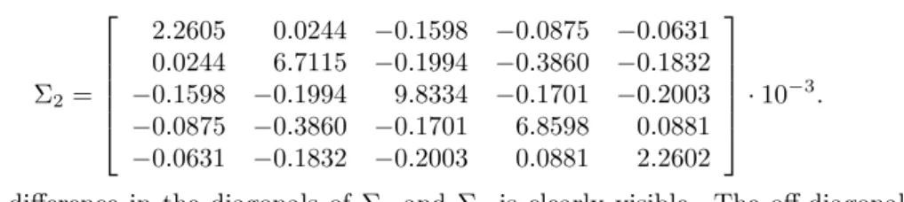
We calculated the empirical covariance matrices Σ1 (corresponding to band- widthh1) andΣ2 (corresponding to bandwidthh2) for our estimators
(fbn(x1), . . . ,fbn(x5)).
Σ1=
0.3078 0.0516 −0.1107 −0.1475 −0.0624 0.0516 0.8053 −0.1524 −0.3343 −0.1540
−0.1107 −0.1524 0.9289 −0.1485 −0.1221
−0.1475 −0.3343 −0.1485 0.7853 0.0632
−0.0624 −0.1540 −0.1221 0.0632 0.3195
·10−3;
Σ2=
2.2605 0.0244 −0.1598 −0.0875 −0.0631 0.0244 6.7115 −0.1994 −0.3860 −0.1832
−0.1598 −0.1994 9.8334 −0.1701 −0.2003
−0.0875 −0.3860 −0.1701 6.8598 0.0881
−0.0631 −0.1832 −0.2003 0.0881 2.2602
·10−3. The difference in the diagonals of Σ1 and Σ2 is clearly visible. The off-diagonal elements are almost the same.
x -1.0 -0.5 0.0 0.5 1.0
f(x) 0.1549 0.4746 0.6892 0.4746 0.1549 fˆn(x)withh1= 0.10 0.1590 0.4726 0.6794 0.4728 0.1599 fˆn(x)withh2= 0.01 0.1543 0.4747 0.6876 0.4763 0.1564
Table 1: Theoretical values of the density function and the average of their estimators for the data of Example 1.
Now calculate the additional terms in the diagonals of the covariance matrices described byΣdefined in Proposition 4.1. In our case the elements of the diagonal matrixVk for the bandwidthhk (k= 1,2) are
1 n
1 hk
f(xi) Z∞
−∞
K2(u)du= 1 2000
1 hk
f(xi) 1 2√π.
Since in the infill-increasing case only the diagonals of the limit covariance matrices can be different for different values of the bandwidth, we show in Table 2 the ratio between the diagonals of the difference of the empirical covariance matrices,diag(Σ2−Σ1), and of the theoretical covariance matrices,diag(V2−V1).
x −1.0 −0.5 0.0 0.5 1.0
diag(Σ2−Σ1)
diag(V2−V1) 0.9927 0.9803 1.0176 1.0082 0.9867 Table 2: Ratio between the diagonal of the difference of the em- pirical covariance matrices and that of the theoretical covariance
matrices for the data of Example 1.
These are close to 1 as it is expected from the above proposition.
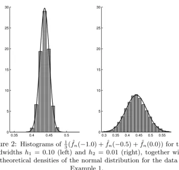
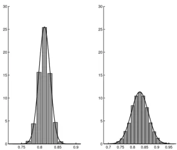
Finally, Figure 1 shows histograms of 12( ˆfn(0.5) + ˆfn(1.0)) for the bandwidths h1 = 0.10(left picture) andh2 = 0.01(right picture). Figure 2 shows histograms of 13( ˆfn(−1.0) + ˆfn(−0.5) + ˆfn(0.0))for the above bandwidths.
The histograms are presented together with the theoretical normal densities with means and variances estimated from the data used for the histograms. The approximate normality of the density estimator stated in the above proposition is reflected in these figures. Different bandwidths lead to different spreads of the normal distribution.
0.25 0.3 0.35 0.4 0
5 10 15 20 25
0.2 0.3 0.4 0.5
0 5 10 15 20 25
Figure 1: Histograms of 12( ˆfn(0.5) + ˆfn(1.0))for the bandwidths h1= 0.10(left) andh2= 0.01(right), together with the theoretical
densities of the normal distribution for the data of Example 1.
0.35 0.4 0.45 0.5
0 5 10 15 20 25 30
0.3 0.35 0.4 0.45 0.5 0.55 0
5 10 15 20 25 30
Figure 2: Histograms of 13( ˆfn(−1.0) + ˆfn(−0.5) + ˆfn(0.0))for the bandwidths h1 = 0.10(left) and h2 = 0.01 (right), together with the theoretical densities of the normal distribution for the data of
Example 1.
Now we consider a two-dimensional domain with fractal-like shape.
Example 2. Two-dimensional moving average.
Now the locations will be the l-lattice points of the domain D = [0, t]2 with l = 0.1 andt = 10. Thus the random field isz(i,j) =ξ(i/10,j/10), i, j = 1, . . . ,100.
Letyk,l,k, l= 1, . . . ,102,be i.i.d. standard normal random variables, and let
z(i,j)= 1 9
Xi+2 k=i
j+2X
l=j
yk,l, i, j= 1, . . . ,100.
Therefore the random field ism-dependent with m= 3. The marginal density is f(x) = √1
2πσexp
−x2 2σ2
where σ= 0.3333.
Some points from the locations were omitted. In Figure 3, the small squares where the locations were deleted are marked with dark. We can see that in each white small square we have 16 sites of observations. Denote the set of the remaining locations byD. So the observations arez(i,j), i, j∈D.Therefore the actual sample size is 7056.
Figure 3: Sampling sites
It can be seen that the resulted domain is not convex. In the above proposition the asymptotic properties of the estimator remain true. It is clearly shown by the following numerical results.
As in the previous example, we calculated the density estimatorfˆnat the points x1 = −1.0, x2 = −0.5, x3 = 0.0, x4 = 0.5, x5 = 1.0. We used the bandwidths
h1 = 0.10 and h2 = 0.01 and applied the standard normal density function as kernelK.The data sets for both bandwidths were the same, and5000repetitions were performed. Table 3 shows that the theoretical values of the density function and the average of their estimators are very similar.
x −1.0 −0.5 0.0 0.5 1.0
f(x) 0.3886 0.9034 1.1968 0.9034 0.3886 fˆn(x) withh= 0.10 0.4087 0.8852 1.1460 0.8858 0.4085 fˆn(x) withh= 0.01 0.3907 0.9032 1.1965 0.9029 0.3895 Table 3: Theoretical values of the density function and the average
of their estimators for the data of Example 2.
The empirical covariance matrices are
Σ1=
0.5124 0.3246 −0.1801 −0.4534 −0.2921 0.3246 0.7406 0.0403 −0.5479 −0.4382
−0.1801 0.0403 0.5769 0.0194 −0.1941
−0.4534 −0.5479 0.0194 0.7785 0.3362
−0.2921 −0.4382 −0.1941 0.3362 0.5089
·10−3;
Σ2=
1.9357 0.2898 −0.1783 −0.5075 −0.2852 0.2898 4.0989 −0.0694 −0.6534 −0.5137
−0.1783 −0.0694 4.9750 −0.1292 −0.2899
−0.5075 −0.6534 −0.1292 4.2037 0.3005
−0.2852 −0.5137 −0.2899 0.3005 1.9322
·10−3 for the bandwidthsh1andh2, respectively. Again, the agreement of the off-diagonal elements and the difference in the diagonal becomes visible.
Similarly to the previous example, we show the ratios diag(Σdiag(V22−Σ−V11)) in Table 4.
These are close to 1 as it was expected from our proposition.
x −1.0 −0.5 0.0 0.5 1.0
diag(Σ2−Σ1)
diag(V2−V1) 1.0181 1.0331 1.0213 1.0537 1.0180 Table 4: Ratio between the diagonal of the difference of the em- pirical covariance matrices and that of the theoretical covariance
matrices for the data of Example 2.
Finally, Figure 4 shows histograms of 12( ˆfn(0.0) + ˆfn(0.5)) for the bandwidths h1 = 0.10(left picture) andh2 = 0.01(right picture). Figure 5 shows histograms of 13( ˆfn(−1.0) + ˆfn(−0.5) + ˆfn(0.0))for the above bandwidths.
The histograms are presented together with the theoretical normal densities with means and variances estimated from the data used for the histograms. The approximate normality of the density estimator stated in the above proposition is reflected in these figures. Different bandwidths lead to different spreads of the normal distribution.
0.95 1 1.05 1.1 0
2 4 6 8 10 12 14 16 18 20 22
0.9 1 1.1 1.2
0 2 4 6 8 10 12 14 16 18 20 22
Figure 4: Histograms of 12( ˆfn(0.0) + ˆfn(0.5))for the bandwidths h1= 0.10(left) andh2= 0.01(right), together with the theoretical
densities of the normal distribution for the data of Example 2.
0.75 0.8 0.85 0.9
0 5 10 15 20 25 30
0.7 0.75 0.8 0.85 0.9 0.95 0
5 10 15 20 25 30
Figure 5: Histograms of 13( ˆfn(−1.0) + ˆfn(−0.5) + ˆfn(0.0))for the bandwidths h1 = 0.10(left) and h2 = 0.01 (right), together with the theoretical densities of the normal distribution for the data of
Example 2.
5. Conclusions
In the paper, the kernel type density estimatorfˆn is considered. The underlying random field ism-dependent but the observation domain can be irregular. Nearly infill sampling scheme is supposed. Based on the CLT of Park, Kim, Park and Hwang [6] the joint asymptotic normality of fˆ1(x1), . . . ,fˆn(xr) is obtained. The asymptotic covariance matrix is unusual in the sense that it is a combination of the covariance matrices in the continuous and the discrete parameter cases. Numerical evidence supports our results.
References
[1] Fazekas, I. and Chuprunov, A. (2004), A central limit theorem for random fields.Acta Mathematica Academiae Paedagogicae Nyiregyhaziensis, 20(1), 93–104, www.emis.de/journals/AMAPN.
[2] Fazekas, I. and Chuprunov, A. (2006), Asymptotic normality of kernel type density estimators for random fields.Stat. Inf. Stoch. Proc.9, 161–178.
[3] Karácsony, Zs. and Filzmoser, P. (2010), Asymptotic normality of kernel type regres- sion estimators for random fields.Journal of Statistical Planning and Inference,140, 872–886.
[4] Lahiri, S.N. (1999), Asymptotic distribution of the empirical spatial cumulative dis- tribution function predictor and prediction bands based on a subsampling method.
Probab. Theory Related Fields,114(1), 55–84.
[5] Lahiri, S.N., Kaiser, M.S., Cressie, N. and Hsu, N.J. (1999), Prediction of spatial cu- mulative distribution functions using subsampling.J. Amer. Statist. Assoc.94(445), 86–110.
[6] Park, B.U., Kim, T.Y., Park, T.-S., Hwang, S.Y. (2009), Practically Applicable Cen- tral Limit Theorem for Spatial Statistics.Math. Geosci.41, 555–569.