Introductory Course in Analysis

(1)

INTRODUCTORY COURSE IN ANALYSIS

(2)

Undergraduate Mathematics

Algoritmuselm´elet

Algoritmusok bonyolults´aga

Analitikus módszerek a pénzügyben és a közgazdaságtanban Anal´ızis feladatgy˝ujtemény I

Anal´ızis feladatgy˝ujtem´eny II Bevezet´es az anal´ızisbe Complexity of Algorithms Differential Geometry

Diszkrét matematikai feladatok Diszkrét optimalizálás

Geometria

Igazs´agos eloszt´asok

Introductory Course in Analysis Mathematical Analysis – Exercises I

Mathematical Analysis – Problems and Exercises II Mértékelmélet és dinamikus programozás

Numerikus funkcionálanal´ızis Operációkutatás

Operációkutatási példatár Parciális differenciálegyenletek Példatár az anal´ızishez Pénzügyi matematika Szimmetrikus struktúrák Többváltozós adatelemzés

Variációszám´ıtás és optimális irány´ıtás

(3)

István Faragó Ágnes Havasi István Mezei Péter Simon

INTRODUCTORY COURSE IN ANALYSIS

Eötvös Loránd University Faculty of Science

Typotex 2014

(4)

Dr. Péter Simon, Eötvös Loránd University, Faculty of Science Reader: Dr. Bálint Nagy

Creative Commons NonCommercial-NoDerivs 3.0 (CC BY-NC-ND 3.0) This work can be reproduced, circulated, published and performed for noncommercial purposes without restriction by indicating the author’s name, but it cannot be modified.

ISBN 978 963 279 223 1

Prepared under the editorship of Typotex Publishing House (http://www.

typotex.hu)

Responsible manager: Zsuzsa Votisky Technical editor: József Gerner

Made within the framework of the project Nr. TÁMOP-4.1.2-08/2/A/KMR- 2009-0045, entitled “Jegyzetek és példatárak a matematika egyetemi oktatá- sához” (Lecture Notes and Workbooks for Teaching Undergraduate Mathe- matics).

KEY WORDS: Mathematical analysis, sets, real and complex numbers, sequences, series, differentiation, integration, analysis of functions, series of functions, vector analysis.

SUMMARY: This textbook has been written for the analysis education of non-mathematics students at the Eötvös Loránd University, Faculty of Sci- ence, but it can also be used as a supplementary material by students of mathematics. All subjects are presented at beginners’ level, where mainly methods are taught. The book is strongly application-oriented. For example, vector calculus is included for students of geophysics, and contour and surface integrals are presented for physics student.

(5)

Preface

These lecture notes are based on the series of lectures that were given by the authors at the Eötvös Loránd University for students in Physics, Geophysics, Meteorology and Geology. It is written firstly for these students, however, it can be also used by students in mathematics. People at the Department of Applied Analysis and Computational Mathematics have taught mathematics to science students for decades. The authors have taken part in this work for several years, they taught the topics dealt with in these lecture notes in many semesters. Their long term teaching and pedagogical experience is behind this work.

Concerning its contents the book is similar to other analysis textbooks, however, it is special because of several reasons. First of all, most of the textbooks are written for students in mathematics, or for non-mathematics students in some special field, for example students in engineering or econ- omy. These lecture notes are customized to science students at the Eötvös Loránd University. According to our teaching experience the students do not acquire mathematical knowledge through the axiomatic set-up, instead they understand mathematical notions and methods gradually getting deeper and deeper synthesis. Hence the lecture notes follow an alternative way, all subjects are presented at the beginners level, when mainly methods are taught (for physics students this corresponds to the Calculus course). The book is strongly application oriented. For example, vector calculus is included for students in geophysics, complex functions, contour and surface integral is presented for physics student.

1

(10)

Acknowledgement

The authors are grateful to their colleagues at the Department of Applied Analysis and Computational Mathematics in the Institute of Mathematics at the Eötvös Loránd University, who supported the creation of the analysis course for science students at the University, and encouraged the efforts to make lecture notes electronically available to the students of these courses.

The authors appreciate the careful work of the referee, Bálint Nagy, who provided detailed comments, identified errors and typos, and helped to in- crease distinctness and consistency of the notes.

(11)

Chapter 2

Sets, relations, functions

We present the tools and frequently used notions of mathematics, and introduce some important conventions. We prepare a solid base for the further constructions. To abbreviate the words “every” or “arbitrary” we will often use the symbol∀, while the notation∃ will be employed for the expression

“exists” or “there is”. This chapter covers the following topics.

• Sets and operations on sets

• Relations

• Functions and their properties

• Composition and inverse functions

2.1 Sets, relations, functions

2.1.1 Sets and relations

Asetis considered as given if we can decide about every well-defined object whether it belongs to the set or not. (A “clever thought”, a “beautiful girl”, a

“sufficiently big number” or a “small positive number” cannot be considered as well-defined objects, so we will not ask if they belong to a set.)

LetAbe a set, and xa well-defined object. Ifxbelongs to the set, then we will denote this asx∈A. If xdoes not belong to the set, we will write x /∈A.

A set can be given by listing its elements, e.g., A := {a, b, c, d}, or by specifying a property, e.g.,B:={x|xis a real number andx²<2}.

Definition 2.1. LetAandB be sets. We say thatAis a subset of B if for allx∈A x∈B holds. Notation: A⊂B.

3

(12)

Definition 2.2. LetAandB be sets. SetA is equal to setB if both have the same elements. Notation: A=B.

It is easy to see that the following theorem holds.

Theorem 2.1. Let AandB be sets. ThenA=B if and only ifA⊂B and B⊂A.

We will show some procedures which yield further sets.

Definition 2.3. LetAandB be sets.

The union ofAandB is the setA∪B:={x|x∈Aor x∈B}.

The intersection ofAandB is the setA∩B:={x|x∈Aandx∈B}.

The difference ofAandB is the set A\B:={x|x∈Aandx /∈B}.

When taking the intersection or the difference of sets, it can happen that no objectxpossesses the required property. The set to which no well-defined object belongs is calledempty set. Notation: ∅.

LetH be a set and A⊂H a subset. The complement ofA(with respect to setH) is defined as the setA:=H\A. The following theorem is known as De Morgan’s identities.

Theorem 2.2. Let H be a set,A, B⊂H. Then we have A∪B=A∩B and A∩B =A∪B.

Let a and b be any objects. The set {a, b} can obviously be written in several ways:

{a, b}={b, a}={a, b, b, a}={a, b, b, a, b, b}=etc.

As opposed to this, we introduce the basic notion of theordered pair(a, b), an essential property of which is

(a, b) = (c, d)if and only if a=candb=d.

We define the product of sets with the aid of ordered pairs.

Definition 2.4. LetA, B be sets. TheCartesian product ofAand B is the set of ordered pairs

A×B:={(a, b)|a∈Aandb∈B}.

For example, letA:={2,3,5} andB:={1,3}, then

A×B ={(2,1),(2,3),(3,1),(3,3),(5,1),(5,3)}.

(13)

2.1. Sets, relations, functions 5 Relations are based on the notion of ordered pair.

Definition 2.5. We say that a setris arelationif each of its elements is an ordered pair.

A Hungarian-English dictionary is a relation because its elements are ordered pairs of a Hungarian word and the corresponding English word.

Definition 2.6. Letrbe a relation. Thedomain of definitionofr is D(r) :={x|there exists any such that(x, y)∈r}.

Therange ofris

R(r) :={y| there exists anx∈D(r)such that(x, y)∈r}.

Obviously,r⊂D(r)×R(r).

For example, in the case of r := {(4,2),(4,3),(1,2)}, D(r) = {4,1}, R(r) ={2,3}.

2.1.2 Functions

A function is a special relation.

Definition 2.7. Letf be a relation. We say thatf is afunctionif for all (x, y)∈f and(x, z)∈f y=z.

For example, r := {(1,2),(2,3),(2,4)} is not a function since (2,3) ∈ r and(2,4)∈r, but36= 4; however,f :={(1,2),(2,3),(3,3)}is a function.

We introduce some conventions in connection with functions. If f is a function, then in case of (x, y)∈ f we call y the valueof function f at x, and we say thatf associatesyto xor maps xtoy. Notation: y=f(x).

Iff is a function,A:=D(f), andB is such a set thatR(f)⊂B (clearly, A is the domain of definition of the function, and B is (a) range of the function, then instead of the expression “f ⊂ A×B, f is a function” the notationf :A→B is employed (“the functionf maps set Ato setB”).

If f is a function and D(f) ⊂ A, R(f) ⊂ B, then this is denoted by f :AB (“f is a function that maps fromsetAto setB”).

For examplef :={(a, α),(b, β),(g, γ),(d, δ),(e, ε)}is a function. One can see thatβ is the value of f atb: β=f(b).

If L denotes the set of Latin letters and G the set of Greek letters, then f :{a, b, g, d, e} →G, f(a) =α, f(b) =β, f(g) =γ, f(d) =δ, f(e) =ε. If we only want to refer to the type of the function, then it is sufficient to write f ∈LG.

Obviously, any function has an inverse, however, it can happen that the inverse is not a function.

(14)

Definition 2.8. Let f : A → B be a function. We say that f is one-to one (injective) if it associates different elements of B to different elements x1, x2∈A, that is, for all x1, x2∈A, x16=x2: f(x1)6=f(x2).

It is easy to see that the inverse of a one-to-one function is a function. In more detail:

Theorem 2.3. Let f be a function, A := D(f), B := R(f), f one-to-one.

Then the inversef⁻¹ :B →A of f is such a function that maps any point s∈B tot∈A for whichf(t) =s, (briefly: for any s∈B: f(f⁻¹(s)) =s).

We can also prepare the composition of functions. Fortunately, it will always be a function.

Letg : A →B, f : B →C. Then by using the composition of relations one can show that

f ◦g:A→C, and for allx∈A: (f ◦g)(x) =f(g(x)).

For example, let the functiongadd 1 to the double of each number (g:R→R, g(x) := 2x+ 1); and the function f raise each number to the second power (f :R→R, f(x) :=x²), then f◦g :R→R,(f ◦g)(x) = (2x+ 1)² will be the composition off andg.

Further useful notions

Letf :A→B and C⊂A. Therestriction of a function f to C is the functionf_|_C :C→B for whichf_|_C(x) :=f(x)for allx∈C.

Letf :A→B, C ⊂AandD⊂B. The set

f(C) :={y| there exists x∈C, such thatf(x) =y}

is called the “image of setC under the functionf”. The set f⁻¹(D) :={x|f(x)∈D}

is called the “preimage of set D under the function f”. (Attention! The notationf⁻¹does not stand for the inverse function in this case.)

2.2 Exercises

1. LetA:={2,4,6,3,5,9},B:={4,5,6,7},H :={n|nis a whole number, 1 ≤n≤20}. Prepare the sets A∪B, A∩B, A\B, B\A. What is the complement of Awith respect toH?

2. LetA:={a, b},B:={a, b, c}. A×B=?B×A=?

(15)

2.2. Exercises 7 3. Letr :={(x, y)|x, yreal numbers,y =x²}. r⁻¹=? Isr a function? Is

r⁻¹a function?

4. Letf :R→R, f(x) := _1+x^x2. Prepare the functionsf◦f,f◦(f◦f).

5. Think over how the inverse of a one-to-one function f : A → B can be illustrated.

6. Consider that the inverse of a functionf :A→B can be obtained in the following steps:

1) Write thaty=f(x).

2) Swap the “variables” xandy: x=f(y).

3) From this equation express y with the aid ofx: y=g(x). This veryg will be the inverse functionf⁻¹.

Example: f :R→R,f(x) = 2x−1. (This is a one-to-one function.) 1)y= 2x−1

2)x= 2y−1

3)x+ 1 = 2y,y= ¹₂(x+ 1).

Sof⁻¹:R→R,f⁻¹(x) =¹₂(x+ 1).

Draw the graphs of the functionsf andf⁻¹. 7. Letf :A→B,C1, C2⊂A, D1, D2⊂B. Show that

f(C₁∪C₂) =f(C₁)∪f(C₂), f(C₁∩C₂)⊂f(C₁)∩f(C₂),

f⁻¹(D₁∪D₂) =f⁻¹(D₁)∪f⁻¹(D₂), f⁻¹(D₁∩D₂) =f⁻¹(D₁)∩f⁻¹(D₂).

Is it true thatC₁⊂C₂ impliesf(C₁)⊂f(C₂)?

Is it true thatD1⊂D2impliesf⁻¹(D1)⊂f⁻¹(D2)?

8. Letf :A→B,C⊂A, D⊂B.

Is it true thatf⁻¹(f(C)) =C? Is it true thatf(f⁻¹(D)) =D?

(16)

(17)

Chapter 3

Sets of numbers

We can calculate with real numbers since our childhood, we add, multiply and divide them, raise them to powers and take their absolute values. We re-arrange equations and inequalities. Now we lay down the relatively simple set of rules from which the learnt procedures can be derived. We will cover the following topics.

• The set of real numbers

• The set of natural numbers

• The sets of integers and rational numbers

• Upper bound, lower bound

• Interval and neighborhood

• Exponentiation and power law identities

• The set of complex numbers

• The trigonometric form of complex numbers, operations

3.1 Real numbers

3.1.1 The axiomatic system of real numbers

LetRbe a nonempty set. Suppose there is a function+ :R×R→Rcalled addition and a function · : R×R →R called multiplication satisfying the following properties:

a1. for alla, b∈R, a+b=b+a(commutativity);

a2. for alla, b, c∈R,a+ (b+c) = (a+b) +c (associativity);

9

(18)

a3. there exists an element0∈Rsuch that for alla∈R, a+ 0 =a(0is a neutral element with respect to addition);

a4. for alla∈Rthere is an element −a∈Rsuch thata+ (−a) = 0;

m1. for alla, b∈R, a·b=b·a;

m2. for alla, b∈R, a·(b·c) = (a·b)·c;

m3. there exists an element1∈Rsuch that for alla∈R, a·1 =a(1is a neutral element with respect to the multiplication);

m4. for alla ∈R\ {0} there exists a reciprocal element ¹_a ∈R for which a· ¹_a = 1;

d. for alla, b, c∈R,a·(b+c) =ab+ac(multiplication is distributive with respect to addition).

It is easy to see that the fourth requirement of multiplication is essentially different from the laws of addition (otherwise the two operations would not differ from each other).

Axiom d also emphasizes the difference.

Assume that there exists an ordering relation≤(called less than or equal to) onR, which has the following further properties:

r1. for alla, b∈Reithera≤b, or b≤aholds;

r2. in all cases wherea≤b andc∈Rare arbitrary numbers,a+c≤b+c;

r3. in all cases where0≤aand0≤b,0≤ab.

Let us fix that instead ofa≤b, a6=b the notationa < bwill be employed.

(Unfortunately, < is not an ordering relation, since it is not reflexive.) On the basis of a1–a4, m1–m4, d, r1–r3 one can derive all “laws” related to equalities and inequalities. As a supplement, we mention three notions.

Definition 3.1. Leta, b∈R,b6= 0. Then ^a_b :=a·¹_b. So, division can be performed with real numbers.

Definition 3.2. Letx∈R. Theabsolute valueofxis

|x|:=

x if 0≤x

−x if x≤0, x6= 0.

Inequalities with absolute value are very useful.

1. For allx∈R,0≤ |x|.

(19)

3.1. Real numbers 11 2. Letx∈Randε∈R, 0≤ε. Thenx≤ε and −x≤ε⇐⇒ |x| ≤ε.

3. For alla, b∈R,|a+b| ≤ |a|+|b|(triangle inequality).

4. For alla, b∈R,||a| − |b|| ≤ |a−b|.

These statements are simple to prove. Here we show the proof of A 4.

Consider the equalitya=a−b+b. Then, by property 3,

|a|=|a−b+b| ≤ |a−b|+|b|.

According to r2, by adding the number−|b|to both sides, the inequality does not change.

|a|+ (−|b|) =|a| − |b| ≤ |a−b|. (3.1) Similarly,

b=b−a+a,

|b|=|b−a+a| ≤ |b−a|+|a| /− |a|,

|b| − |a| ≤ |b−a|,

−(|a| − |b|)≤ |b−a|=|a−b|. (3.2) The inequalities (3.1) and (3.2) according to property 2 (by the choicex:=

|a| − |b|;ε:=|a−b|) exactly yield||a| − |b|| ≤ |a−b|.

3.1.2 Natural, whole and rational numbers

Now we separate a famous subset ofR. LetN⊂Rbe such a subset for which 1^o 1∈N,

2^o for alln∈N,n+ 1∈N,

3^o for alln∈N,n+ 16= 1(1 is the “first” element), 4^o the facts that a)S⊂N,

b)1∈S,

c) for alln∈S,n+ 1∈S implyS =N. (Complete induction.)

This subsetNofRis called the set of natural numbers.

We supplement all this with the following definitions:

Z:=N∪ {0} ∪ {m∈R| −m∈N} isthe set of integers,

Q :={x∈ R | there exists p∈ Z, q ∈ Nsuch thatx = ^p_q} is the set of rational numbers,

(20)

Q^∗:=R\Qisthe set of irrational numbers.

With the aid of N, we impose a third requirement on R in addition to the laws of the operations and ordering.

Archimedes’ axiom: For all a, b ∈ R, 0 < athere exists n ∈ N such thatb < na.

As a consequence of Archimedes’ axiom, one can show that for allK∈R there exists a natural number n∈ Nfor which K < n, since by the choice a:= 1,b:=Kthe axiom provides such a natural number.

We also show that for allε∈R,0< εthere exists a natural numbern∈N such that _n¹ < ε, since let us choose a := ε and b := 1. According to the axiom there is an n∈ N such that 1 < n·ε. By applying the appropriate

“law”:

1< nε /+ (−1), 0< nε−1 /· 1

n, 0< 1

n(nε−1) =ε− 1

n /+ 1 n, 1

n < ε.

Even with the introduction of Archimedes’ axiom R does not meet all de- mands. We need a final axiom, for which we make preparations by introduc- ing some further notions.

3.1.3 Upper and lower bound

Definition 3.3. Let A ⊂ R, A 6= ∅. We say that the set A is bounded aboveif there exists aK∈Rsuch that for alla∈A,a≤K. Such a number Kis called an upper boundof setA.

LetA⊂R, A6=∅ be bounded above. Consider

B:={K∈R|Kis an upper bound of setA}.

Letα∈Rbe the smallest element of setB, that is, a number for which 1^oα∈B (αis an upper bound of setA),

2^ofor all upper bounds K∈B,α≤K.

The only question is whether there exists such anα∈R.

The least upper bound axiom: Every setA⊂R, A6=∅of real numbers having an upper bound must have a least upper bound.

(21)

3.1. Real numbers 13 Such a numberα∈R(which is not necessarily an element ofA) is called supremumofAand denoted as

α:= supA.

Clearly, the following two properties ofsupAhold:

1^ofor alla∈A,a≤supA,

2^ofor all0< εthere exists a⁰∈Asuch that(supA)−ε < a⁰.

The laws of the operations and ordering, Archimedes’ axiom and the least upper bound axiom make the set of real numbers Rcomplete. In this way we have laid down a solid base for the future calculations, too.

Some further conventions:

Definition 3.4. LetA ⊂R, A6=∅. We say thatA is bounded belowif there exists anL∈Rsuch that for alla∈A,L≤a. The numberLis called (a) lower bound of setA.

Let A be a set of numbers that is bounded below. The greatest lower bound ofAis calledinfimumofA. (The existence of this lower bound does not require any new axiom, it follows from the least upper bound axiom.) The infimum ofAis denoted as

infA.

Obviously,

1^ofor alla∈A,infA≤a,

2^ofor all0< εthere exists ana⁰ ∈Asuch thata⁰<(infA) +ε.

3.1.4 Intervals and neighborhoods

Definition 3.5. LetI⊂R. We say thatIis anintervalif for allx₁, x₂∈I, x₁< x₂: anyx∈Rfor whichx₁< x < x₂ is in I.

Theorem 3.1. Let a, b∈R, a < b.

[a, b] :={x∈R|a≤x≤b}, [a, b) :={x∈R|a≤x < b}, (a, b] :={x∈R|a < x≤b}, (a, b) :={x∈R|a < x < b},

(22)

[a,+∞) :={x∈R|a≤x},

(a,+∞) :={x∈R|a < x};(0,+∞) =:R⁺, (−∞, a] :={x∈R|x≤a},

(−∞, a) :={x∈R|x < a};(−∞,0) =:R⁻, (−∞,+∞) :=R.

All these are intervals. We mention that [a, a] = {a} and (a, a) = ∅ are degenerate intervals.

Definition 3.6. Let a ∈ R, r ∈ R⁺. The neighborhood with radius r of pointais defined as the open interval

Kr(a) := (a−r, a+r).

We say thatK(a)is aneighborhood of point aif there exists an r∈R⁺ such thatK(a)⊂K_r(a).

3.1.5 The powers of real numbers

Definition 3.7. Leta∈R. Thena¹:=a, a²:=a·a, a³:=a²·a, . . . , aⁿ:=

aⁿ⁻¹·a, . . .

Definition 3.8. Leta∈R, 0≤a. Denote by √

athe nonnegative number whose square isa, i.e.,0≤√

a, (√

a)²=a.

Note that for alla∈R,√

a²=|a|.

Definition 3.9. Leta∈R, k∈N. Denote by ^2k+1√

athe real number whose (2k+ 1)th power isa.

Note that if0< a, then ^2k+1√

a >0, and ifa <0, then ^2k+1√ a <0.

Definition 3.10. Leta∈R,0≤a, k ∈N. Denote by ^2k√

athe nonnegative number whose(2k)th power isa.

Let us introduce the following notation: ifn∈N anda∈Rcorresponds to the parity ofn, then

aⁿ¹ := √ⁿ a.

Definition 3.11. Leta∈R⁺, p, q∈N. a^p^q :=√^q

a^p.

(23)

3.2. Exercises 15 Definition 3.12. Leta∈R⁺, p, q∈N.

a⁻^p^q := 1

√q

a^p. Definition 3.13. Leta∈R\ {0}. Thena⁰:= 1.

By this chain of definitions we have defined the numbera∈R⁺ raised to any rational powerr∈Q. One can show that the numbers in the definitions uniquely exist, and the following identities are valid:

1ôfora∈R⁺,r, s∈Q,a^r·a^s=a^r+s, 2ôfora∈R⁺,r∈Q,a^r·b^r= (ab)^r, 3ôfora∈R⁺,r, s∈Q,(a^r)^s=a^rs.

3.2 Exercises

1. Leta, b∈R. Show that

(a+b)²: = (a+b)(a+b) =a²+ 2ab+b², a²−b²= (a−b)(a+b),

a³−b³= (a−b)(a²+ab+b²), a³+b³= (a+b)(a²−ab+b²) 2. Prove that for allx∈R,x6= 1andn∈N

xⁿ⁺¹−1

x−1 = 1 +x+x²+· · ·+xⁿ. 3. (Bernoulli’s inequality)

Leth∈(−1,+∞)andn∈N. Show that (1 +h)ⁿ ≥1 +nh.

Solution: LetS:={n∈N|(1 +h)ⁿ≥1 +nh}.

1^o 1∈S, since(1 +h)¹= 1 + 1·h.

2^o Letk∈S. Thenk+ 1∈S, since

(1 +h)^k+1= (1 +h)^k(1 +h)≥(1 +kh)(1 +h) =

= 1 + (k+ 1)h+kh²≥1 + (k+ 1)h.

(24)

(In addition to the rules of ordering we have exploited the fact that k∈S, that is,(1 +h)^k ≥1 +kh.)

Keeping in mind requirement 4^o during the introduction of N, this means that S=N, so the inequality holds for alln∈N. This method of proof is calledmathematical induction.

4. Leta, b∈R⁺. A₂:= a+b

2 , G₂:=√

ab, H₂:= 2

1

a+¹_b, N₂:=

ra²+b² 2 . Show that H2 ≤ G2 ≤ A2 ≤ N2, and there is equality between the numbers if and only ifa=b.

These equalities are also valid in a more general case.

Letk∈N(k≥3)andx1, x2, . . . , xk ∈R⁺. A_k :=x1+x2+· · ·+xk

k , G_k:= √^k

x₁x₂· · ·x_k,

H_k := k

1 x1 +_x¹

2 +· · ·+_x¹

k

, N_k:=

rx²₁+x²₂+· · ·+x²_k

k .

One can show thatH_k ≤G_k ≤A_k≤N_k, and there is equality between the numbers if and only ifx₁=x₂=. . .=x_k.

5. Leth∈Randn∈N. Then (1 +h)ⁿ = 1 +nh+

n 2

h²+ n

3

h³+· · ·+hⁿ, where, exploiting the fact thatk! := 1·2·. . .·k,

n k

= n!

k!(n−k)!, k= 0,1,2, . . . , n (remember that0! := 1).

From this, one can prove the binomial theorem:

Leta, b∈R, n∈N. Then (a+b)ⁿ=

n

X

k=0

n k

a^kb^n−k.

(25)

3.2. Exercises 17 6. LetA:=n

n

n+1 |n∈N o

. Show thatAis bounded above. FindsupA.

Solution: Since for alln∈N,n < n+ 1, therefore _n+1ⁿ <1, soK:= 1 is an upper bound. We show thatsupA= 1, since

1^o For alln∈N, _n+1ⁿ <1.

2^o Letε∈R⁺. We seek such an indexn∈Nfor which n

n+ 1 >1−ε,

n >(1−ε)(n+ 1) =n−εn+ 1−ε, εn >1−ε,

n < 1−ε ε .

Since one can find a greater natural number than any real number, there is a greater natural number than ^1−ε_ε ∈Ras well, let it ben⁰∈N, therefore for _nⁿ0+1⁰ ∈A, _nⁿ0+1⁰ >1−ε. SosupA= 1.

7. * LetE:={(ⁿ⁺¹_n )ⁿ |n∈N}. Show thatE⊂Ris bounded above.

Solution: We show that for alln∈N n+ 1

n n

≤4.

Letn∈N, and consider the number¹₄(ⁿ⁺¹_n )ⁿ. According to the equality between the algebraic (A_k) and geometric (G_k) means in Exercise 4:

1 4

n+ 1 n

n

=1 2 ·1

2 ·n+ 1 n ·n+ 1

n · · ·n+ 1

n ≤

≤ 1

2+¹₂+ⁿ⁺¹_n +ⁿ⁺¹_n . . .ⁿ⁺¹_n n+ 2

ⁿ⁺²

= 1,

thus (ⁿ⁺¹_n )ⁿ ≤4, and so E is bounded above. According to the least upper bound axiom ithasa supremum. Lete:= supE.

We remark that this supremum has never been and will never be con- jectured (as opposed to Exercise 6...). It is approximately e ≈ 2.71.

The numberewas introduced by Euler.

8. Let P :=

1−1

2

·

1− 1 2²

·

1− 1 2³

· · ·

1− 1 2ⁿ

|n∈N

. Is there aninfP? (When you have shown thatinfP exists, do not get disappointed if you cannot find it. The problem is unsolved.)

(26)

3.3 Complex numbers

3.3.1 The concept of complex numbers, operations

We generalize the real numbers in such a way that the properties of the operations remain unchanged.

LetC:=R×Rthe set of real ordered pairs. Introduce the addition for any(a, b),(c, d)∈Cas

(a, b) + (c, d) := (a+c, b+d);

and the multiplication as

(a, b)·(c, d) := (ac−bd, ad+bc).

It is easy to check some properties of addition and multiplication.

a1. ∀(a, b),(c, d)∈C,(a, b) + (c, d) = (c, d) + (a, b)(commutativity).

a2. ∀(a, b),(c, d),(e, f)∈C,(a, b) + ((c, d) + (e, f)) = ((a, b) + (c, d)) + (e, f) (associativity).

a3. ∀(a, b)∈C,(a, b) + (0,0) = (a, b).

a4. ∀(a, b)∈C,(−a,−b)∈Cis such that(a, b) + (−a,−b) = (0,0).

m1. ∀(a, b),(c, d)∈C,(a, b)·(c, d) = (c, d)·(a, b)(commutativity).

m2. ∀(a, b),(c, d),(e, f) ∈ C, (a, b)·((c, d)·(e, f)) = ((a, b)·(c, d))·(e, f) (associativity).

m3. ∀(a, b)∈C,(a, b)·(1,0) = (a, b).

m4. ∀(a, b)∈C\ {(0,0)},(_a₂_+b^a ₂,−_a2+b^b ²)∈Cis such that (a, b)·

a

a²+b²,− b a²+b²

= (1,0).

d. ∀(a, b),(c, d),(e, f)∈C

(a, b)·[(c, d) + (e, f)] = (a, b)·(c, d) + (a, b)·(e, f) (multiplication is distributive with respect to addition).

(27)

3.3. Complex numbers 19 The properties a1–a4, m1–m4 and d ensure that operations and calculations performed with real numbers (containing only addition and multiplication and referring only to equalities) can be performed with complex numbers in the same way.

Let us identify the real numbera∈Rand the complex number(a,0)∈C. (Clearly, there is a one-to-one correspondence between Rand the complex setR× {0} ⊂C.) We introduce theimaginary unit i:= (0,1)∈C. Then for all complex number(a, b)∈C

(a, b) = (a,0) + (0,1)(b,0) =a+ib.

(The second equality is the consequence of the identification!)

Taking into account thati² = (0,1)·(0,1) =−1, the addition becomes simple:

a+ib+c+id=a+c+i(b+d), and so does the multiplication:

(a+ib)·(c+id) =ac−bd+i(ad+bc).

Complex numbers can be illustrated as position vectors (Fig. 3.1).

1 a

i

b (a,b)=a+ib

•

Figure 3.1

Addition corresponds to the addition of vectors in the plane by the “par- allelogram rule” (Fig. 3.2).

3.3.2 The trigonometric form of complex numbers

To a complex number a+ib ∈ C we can assign its absolute value and its direction angle (Fig. 3.3).

(28)

a+ib c+id

a+c+i(b+d)

•

Figure 3.2

a

b a+ib

r

φ

•

Figure 3.3 The absolute value: r=√

a²+b².

The direction angle can be given in each quarter plane:

φ=











arctg_a^b ifa >0 andb≥0,

π

2 ifa= 0andb >0, π−arctg|^b_a| ifa <0 andb≥0, π+ arctg|^b_a| ifa <0 andb <0,

3π

2 ifa= 0andb <0, 2π−arctg|_a^b| ifa >0 andb <0.

One can see that for the direction angle φ ∈ [0,2π). We remark that for a= 0, b= 0: r= 0, and the direction angle is arbitrary.

(29)

3.3. Complex numbers 21

•

β α α+β

r p

rp

Figure 3.4

If a complex numbera+ib∈Chas absolute vale rand direction angleφ, then

a=rcosφ, b=rsinφ,

therefore,a+ib=r(cosφ+isinφ). This is the trigonometric formof a complex number. With the aid of the trigonometric form the multiplication of complex numbers becomes geometrically meaningful.

Letr(cosα+isinα), p(cosβ+isinβ)∈C, then r(cosα+isinα)· p(cosβ+isinβ) =

=rp(cosαcosβ−sinαsinβ+i(sinαcosβ+ cosαsinβ)) =

=rp(cos(α+β) +isin(α+β)).

So, by multiplication the absolute values are to be multiplied, and the direction angles to be added (Fig. 3.4).

Exponentiation also becomes fairly simple with the trigonometric form. If z=a+ib=r(cosφ+isinφ)∈Candn∈N, then

zⁿ = (a+ib)ⁿ= [r(cosφ+isinφ)]ⁿ=rⁿ(cosnφ+isinnφ),

so, when raising a complex numberzto thenth power, thenth power of the absolute value andntimes the direction angle are taken in the trigonometric form ofzⁿ.

(30)

(31)

Chapter 4

Elementary functions

We present the major properties of functions defined on and mapping to the set of real numbers. We define the frequently used real functions called elementary functions. The following topics will be covered.

• Operations on real functions

• Bounded, monotone, periodic, odd and even functions

• Power functions

• Exponential and logarithmic functions

• Trigonometric functions and their inverses

• Hyperbolic function and their inverses

• Some peculiar functions

4.1 The basic properties of real functions

Definition 4.1. Letf :R⊃→R, λ∈R.Then

λf:D(f)→R, (λf)(x) :=λf(x).

Definition 4.2. Letf, g:R⊃→R, D(f)∩D(g)6=∅. Then f+g:D(f)∩D(g)→R, (f+g)(x) :=f(x) +g(x),

f·g:D(f)∩D(g)→R, (f ·g)(x) :=f(x)·g(x).

Definition 4.3. Letg :R⊃→R, H :=D(g)\ {x∈D(g)|g(x) = 0} 6=∅.

Then

1/g:H →R, (1/g)(x) := 1 g(x). 23

(32)

Definition 4.4. Letf, g:R⊃→R f

g :=f·1/g

Definition 4.5. Letf :R⊃→R. We say thatf isbounded aboveif the setR(f)⊂Ris bounded above.

We say thatf isbounded belowif the setR(f)⊂Ris bounded below.

We say that f is a bounded function if the set R(f) ⊂ R is bounded below and above.

Definition 4.6. Letf : R⊃→ R. We say thatf is a monotonically in- creasingfunction if for allx1, x2∈D(f), x1< x2: f(x1)≤f(x2).

The functionf is strictly monotonically increasingif for allx1, x2∈ D(f),x1< x2: f(x1)< f(x2).

We say thatf is amonotonically decreasingfunction if for allx1, x2∈ D(f),x1< x2: f(x1)≥f(x2).

The functionf isstrictly monotonically decreasingif for allx1, x2∈ D(f),x1< x2: f(x1)> f(x2).

Definition 4.7. Letf :R⊃→R.We say thatf is anevenfunction if 1^ofor allx∈D(f),−x∈D(f),

2^ofor allx∈D(f),f(−x) =f(x).

Definition 4.8. Letf :R⊃→R.We say thatf is anoddfunction if 1^ofor allx∈D(f),−x∈D(f),

2^ofor allx∈D(f),f(−x) =−f(x).

Definition 4.9. Let f : R⊃→R. We say that f is a periodicfunction if there exists a numberp∈R, 0< psuch that

1^ofor allx∈D(f),x+p, x−p∈D(f), 2^ofor allx∈D(f),f(x+p) =f(x−p) =f(x).

The numberpis called aperiodof the function f.

4.2 Elementary functions

4.2.1 Power functions

Let id:R⊃→R, id(x) :=x.As Fig. 4.1 shows, id is a strictly monotonically increasing function.

(33)

4.2. Elementary functions 25

id

Figure 4.1

id²

1 1

Figure 4.2

(34)

id³

1 1

Figure 4.3

id⁻¹

1 1

Figure 4.4

Let id²:R⊃→R, id²(x) :=x².Clearly, id²_|

R+ is a strictly monotonically increasing function, while id²_|

R− is strictly monotonically decreasing. The function id²is even (Fig. 4.2).

Let id³ : R ⊃→ R, id³(x) := x³. Function id³ is strictly monotonically increasing and odd (Fig. 4.3). If n ∈ N, then the function idⁿ : R → R, idⁿ(x) :=xⁿ inherits the properties of id² for even n, and the properties of id³ for oddn.

Let id⁻¹:R\ {0} →R, id⁻¹(x) := 1/x. The functions id⁻¹_|

R− and id⁻¹_|

R+

are strictly monotonically decreasing (however, id⁻¹is not monotone!). The function id⁻¹ is odd (Fig. 4.4).

(35)

id⁻² 1

1

Figure 4.5

id^1/2

1 1

Figure 4.6

Let id⁻²: R\ {0} →R, id⁻²(x) := 1/x². The function id⁻²_|

R− is strictly monotonically increasing, while id⁻²_|

R+ is strictly monotonically decreasing.

The function id⁻²is even (Fig. 4.5).

Letn ∈N. The function id⁻ⁿ : R\ {0} →R, id⁻ⁿ(x) := 1/xⁿ inherits the properties of id⁻²ifnis even, and those of id⁻¹ ifnis odd.

Let id^1/2: [0,∞)→R, id^1/2(x) :=√

x.The function id^1/2is strictly monotonically increasing (Fig. 4.6). We mention that id^1/2 can also be defined as the inverse of the one-to-one function id²_|_[0,∞).

Let r ∈ Q, and consider the function id^r : R⁺ → R, id^r(x) := x^r. For some values ofrthe functions id^r are plotted in Fig. 4.7.

(36)

id^3/2

id^2/3

id⁰ id^−1/2

1 1

Figure 4.7

Finally, let id⁰ : R → R, id⁰(x) := 1. The function id⁰ is even, monotonically increasing, and at the same time monotonically decreasing. It is periodic by any numberp >0(Fig. 4.7).

4.2.2 Exponential and logarithmic functions

Leta∈R⁺. The exponential function with base ais defined as exp_a :R→R, exp_a(x) :=a^x.

exp_a is strictly monotonically increasing if a >1, exp_a is strictly monotonically decreasing ifa <1,

exp_a =id⁰ ifa= 1 (monotonically increasing and decreasing at the same time) (Fig. 4.8).

Ifa >0 and a6= 1, thenR(exp_a) =R⁺, so exp_a only takes positive values (and it does take all positive values). For alla >0 and by anyx1, x2∈R:

exp_a(x₁+x₂) = exp_a(x₁)·exp_a(x₂).

(This is the most important characteristic of the exponential functions.) A special role is played by the functionexp_e=: exp(Fig. 4.9) (whereeis Euler’s number introduced in Exercise 7* of the previous chapter).

Leta >0, a6= 1. Sinceexp_ais strictly monotone, therefore it is one-to-one, and so it has an inverse function:

log_a:= (exp_a)⁻¹

(37)

expa a>1 expa a<1

exp1 1

Figure 4.8

1 e

exp

Figure 4.9

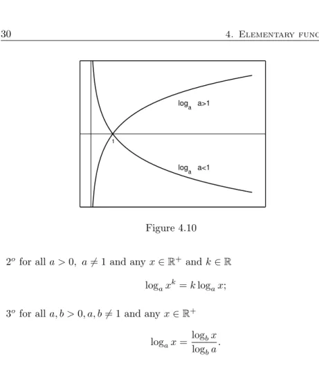
called logarithmic function with basea(Fig. 4.10). So

log_a :R⁺→R, log_a(x) =y, for which exp_a(y) =x.

If a > 1, then log_a is strictly monotonically increasing, and if a < 1, then log_a is strictly monotonically decreasing. Logarithmic functions have the fundamental properties that

1^ofor alla >0,a6= 1 and anyx1, x2∈R⁺

log_a(x₁x₂) = log_ax₁+ log_ax₂;

(38)

loga a>1

loga a<1 1

Figure 4.10 2^ofor alla >0, a6= 1and anyx∈R⁺ andk∈R

log_ax^k =klog_ax;

3^ofor alla, b >0, a, b6= 1and anyx∈R⁺ log_ax= log_bx

log_ba.

Property3^o implies that all logarithmic functions can be obtained by mul- tiplying any one logarithmic function by a real number. That is why the logarithmic function to the basee, called “natural logarithm” plays a special role:

ln := log_e (Fig. 4.11).

4.2.3 Trigonometric functions and their inverses

Letsin :R→R, sinx:=Do not expect a formula here! Draw a circle of radius 1. Then draw two straight lines perpendicular to each other through the center of the circle. One of them will be called axis (1), while the other axis (2). From the point where the (positive half) of axis (1) intersects the circle

“measure the arc corresponding to the numberx∈Rto the circumference”.

[This operation requires considerable manual skills!. . . ] The second coordi- nate of the end pointP of the arc will besinx(Fig. 4.12). The sine function is odd, and periodic with periodp= 2π(Fig. 4.13). R(sin) = [−1,1].

(39)

1 e

ln 1

Figure 4.11

•

1 x

sin x P 1

(1) (2)

Figure 4.12

(40)

sin

π/2 π 2π

1

−1

−π/2

Figure 4.13

cos π/2 π

2π 1

−1

−π/2

Figure 4.14

(41)

tg

−π/2 π/2 π

Figure 4.15

Letcos : R → R, cosx := sin(x+^π₂). The cosine function is even, and periodic with periodp= 2π(Fig. 4.14). R(cos) = [−1,1].

Fundamental relationships:

1^oFor allx∈R, cos²x+ sin²x= 1.

2^oFor allx₁, x₂∈R,sin(x₁+x₂) = sinx₁cosx₂+ cosx₁sinx₂, cos(x1+x2) = cosx1cosx2−sinx1sinx2. Let tg:= ^sin_cos and ctg:= ^cos_sin.

It follows from the definition that D(tg) =R\nπ

2 +kπ|k∈Z o

, D(ctg) =R\ {kπ|k∈Z}.

The functions tg and ctg are odd, and periodic with periodp=π(Fig. 4.15 and Fig. 4.16).

Due to their periodicity, trigonometric functions are not one-to-one functions.

Consider the resrictionsin_|_[−_π

2, π2]. This function is strictly monotonically increasing, therefore one-to-one, and so it has an inverse function:

arcsin := (sin_|_[−π 2, π2])⁻¹.

From the definitionarcsin : [−1,1]→[−^π₂,^π₂], arcsinx=αfor whichsinα= x.

The arcsin function is strictly monotonically increasing and odd (Fig. 4.17).

(42)

ctg

−π/2 π/2 π

−π

Figure 4.16

arcsin π/2

1

−1

−π/2

Figure 4.17

The restriction to the interval[0, π]of the cosine function is strictly monotonically decreasing, therefore it has an inverse function:

arccos := (cos_|_[0,π])⁻¹.

From the definition it follows thatarccos : [−1,1]→[0, π], arccosx=αfor whichcosα=x.

The arccos function is strictly monotonically decreasing (Fig. 4.18).

The restriction to the interval(−^π₂,^π₂)of the tg function is strictly monotonically increasing, therefore it has an inverse function:

arctg:= (sin_|_[−π 2, π2])⁻¹.

(43)

arccos π

1

−1

Figure 4.18

From the definition it follows that arctg: R → (−^π₂,^π₂), arctg x = α for which tgα=x.

The arctg function is strictly monotonically increasing and odd (Fig. 4.19).

arctg π/2

−π/2

Figure 4.19

The restriction to the interval (0, π)of the ctg function is strictly monotonically decreasing, therefore it has an inverse function:

arcctg:= (ctg_|_[0,π])⁻¹.

From the definition it follows that arcctg : R → (0, π), arcctgx = α for which ctgα=x.

The arcctg function is strictly monotonically decreasing (Fig. 4.20).

(44)

arcctg π/2

π

Figure 4.20

sh

Figure 4.21

4.2.4 Hyperbolic functions and their inverses

Let sh : R→ R, shx := ^e^x^−e₂^−x. The sh function is strictly monotonically increasing and odd (Fig. 4.21).

Let ch : R → R, chx := ^e^x^+e₂^−x. The function ch_|

R− is strictly monotonically decreasing, while ch_|

R+ is strictly monotonically increasing. The ch function is even. R(ch) = [1,+∞). This function is often called chain curve (Fig. 4.22).

Fundamental relationships:

1^o For allx∈R, ch²x−sh²x= 1.

(45)

ch

1

Figure 4.22

2^o For allx1, x2∈R

sh(x1+x2) =shx1chx2+chx1shx2, ch(x1+x2) =chx1chx2+shx1shx2. Let th:=_ch^sh, cth:= ^ch_sh.

It follows from the definition that th : R → R, thx = ^e_e^x_x^−e_+e^−x−x, cth : R\ {0} →R, cth x= ^e_ex^x^+e−e^−x^−x. The th and cth functions are odd (Fig. 4.23).

th cth 1

−1

Figure 4.23

The th function is strictly monotonically increasing. R(th) = (−1,1).

(46)

arsh

Figure 4.24 The function cth_|

R− is strictly monotonically decreasing, while cth_|

R+ is strictly monotonically increasing. R(cth) =R\[−1,1].

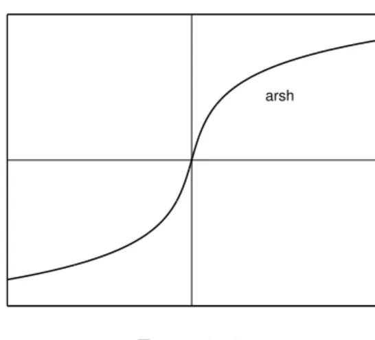
The sh function is strictly monotonically increasing, and so it has an inverse function:

arsh:= (sh)⁻¹.

It follows from the definition that arsh:R→R, arshx= ln(x+√ x²+ 1) (see Exercise 5). The arsh function is strictly monotonically increasing and odd (Fig. 4.24).

The restriction to the interval[0,∞) of the ch function is strictly monotonically increasing, therefore it has an inverse function:

arch:= (ch_|_[0,∞))⁻¹.

From the definition it follows that arch : [1,∞) → [0,∞), archx = ln(x+√

x²−1). The arch function is strictly monotonically increasing (see Fig. 4.25).

The th function is strictly monotonically increasing, so it has an inverse function:

arth:= (th)⁻¹.

From the definition it follows that arth : (−1,1) → R, arth x= ¹₂ln^1+x_1−x. The arth function is strictly monotonically increasing and odd (Fig. 4.26).

The restriction toR⁺ of the cth function is strictly monotonically decreasing, therefore it has an inverse function:

arcth:= (cth_|

R+)⁻¹.

From the definition it follows that arcth: (1,+∞)→R⁺, arcthx=¹₂ln^x+1_x−1. The arcth function is strictly monotonically decreasing (Fig. 4.27).

(47)

arch

1

Figure 4.25

arth

1

−1

Figure 4.26

(48)

arcth

1

Figure 4.27

abs

1 1

Figure 4.28

4.2.5 Some peculiar functions

1. Let abs:R→R, abs(x) :=|x|, where (as we saw before)

|x|:=

x, ifx≥0,

−x, ifx <0 (Fig. 4.28).

2. Let sgn:R→R,sgn(x) :=







1, ifx >0, 0, ifx= 0,

−1, ifx <0

(Fig. 4.29).

(49)

sgn 1

−1

•

Figure 4.29

ent 1

1 2

−1

•

Figure 4.30

3. Let ent:R→R,ent(x) := [x], where

[x] := max{n∈Z|n≤x}.

(The “integer part” of the numberx∈Ris the greatest integer that is less than or equal tox.) (Fig. 4.30.)

4. Letd:R→R, d(x) :=

1 ifx∈Q, 0 ifx∈R\Q.

This function is called Dirichlet’s function, and we do not make an attempt to draw it.

(50)

5. Letr:R→R

r(x) :=

0 ifx∈R\Qorx= 0,

1

q ifx∈Q, x= ^p_q,

wherep∈Z, q∈N, andpandqhave no common divisor (different from 1). It is called Riemann’s function, and again we do not try to plot it.

4.3 Exercises

1. Compute the following function values:

id⁰(7) = id³ 1

2

= id¹²(4) = id⁻⁶(1) = id(6) = id³

−1 2

= id³²(4) = id⁻⁶(2) = id²(5) = id³(0) = id⁻³²(4) = id⁻⁶

1 2

= 2. Arrange the following numbers in ascending order:

a) sin 1, sin 2, sin 3, sin 4;

b) ln 2, exp₂¹₂, exp1

2 2, log₂1;

c) sh3, ch(−2), arsh4, th1;

d) arcsin¹₂, arctg10, th10, cos 1.

3. Prove that ch²x−sh²x= 1, ch²x= ^ch(2x)+1₂ for allx∈R. 4. Prove that forx, y∈R

a) sin 2x = 2 sinxcosx, cos 2x = cos²x−sin²x, cos²x = ^{1+cos 2x}₂ , sin²x= ^{1−cos 2x}₂ ;

b) sinx−siny= 2 sin^x−y₂ cos^x+y₂ , cosx−cosy= 2 sin^y−x₂ sin^x+y₂ . 5. Show that

a) arshx= ln(x+√

x²+ 1) (x∈R);

b) archx= ln(x+√

x²−1) (x∈[1,+∞));

c) arthx= ¹₂ln^1+x_1−x (x∈(−1,1)).

Solution: a)

1^o y=shx= ^e^x^−e₂^−x;

(51)

4.3. Exercises 43 2^o x= ^e^y^−e₂^−y;

2x=e^y−e^−y/·e^y; 2xe^y = (e^y)²−1;

(e^y)²−2xe^y−1 = 0;

(e^y)_1,2= ^2x±

√4x²+4

2 =x±√

x²+ 1.

Since the exp function only takes positive values, and for all x ∈ R

√x²+ 1>√

x²=|x| ≥x, therefore e^y=x+p

x²+ 1.

From this

y= ln(x+p x²+ 1), which means that

3^o arshx= ln(x+p

x²+ 1).

6. Show that arctg6= ^π₂th.

7. Sketch the following functions:

a) f :R→R, f(x) :=

sin¹_x ifx6= 0, 0 ifx= 0.

b) g:R→R, g(x) :=

x²sin_x¹ ifx6= 0, 0 ifx= 0.

c) h:R→R, h(x) :=

x²(sin¹_x+ 2) ifx6= 0, 0 ifx= 0.

8. Let f : R → R be an arbitrary function. Show that for the functions φ, ψ:R→R

φ(x) := f(x) +f(−x)

2 , ψ(x) :=f(x)−f(−x)

2 .

φ is even, ψ is odd, and f = φ+ψ. If f = exp, then what will be the functions φandψ?

9. Let f, g : R → R. Assume that f is periodic with period p > 0, andg with periodq >0.

a) Show that if ^p_q ∈Q, thenf+g is periodic.

b) Give an example where ^p_q ∈R\Q, andf+g is not periodic.

Solution: a) Let ^p_q = ^k_l, wherek, l∈N. Thenlp=kq. Let ω:=lp+kq >

0. We show thatf +gis periodic with periodω.

(52)

1^o D(f+g) =R. 2^o For allx∈R

(f+g)(x+ω) =f(x+kq+lp) +g(x+lp+kq)

=f(x+kq) +g(x+lp) =f(x+lp) +g(x+kq)

=f(x) +g(x) = (f +g)(x).

One can similarly prove that(f +g)(x−ω) = (f+g)(x).

(53)

Chapter 5

Sequences, series

Sequences are fairly simple functions. They are useful in studying the ac- curacy of approximations. They are important building stones of the later concepts. We will deal with the following topics.

• The concept of sequence, monotonicity, boundedness

• Limit and convergence

• Important limits

• The relationships between limits and operations

• The definition of the numbere

• Cauchy’s convergence criterion for sequences

• The convergence of series

• Convergence criteria for series

5.1 Sequences, series

5.1.1 The concept and properties of sequences

A sequence is a function defined on the set of natural numbers.

LetH 6= ∅ be a set. If a: N →H, then we have a sequence inH. For example, ifH is the set of real numbers, then we have a number sequence; if H is a set of certain signals, then we have a signal sequence; ifH is a set of intervals, then we have an interval sequence.

Let a : N → R be a number sequence. If n ∈ N, then we denote the nth element of the sequence by a_n instead of a(n). The number sequence a:N→Rwill also be denoted more briefly as(a_n), or we can emphasize by writing(a_n)⊂Rthat we have a number sequence.

45

Introductory Course in Analysis

INTRODUCTORY COURSE IN ANALYSIS

István Faragó Ágnes Havasi István Mezei Péter Simon

INTRODUCTORY COURSE IN ANALYSIS

Contents

Chapter 1

Preface

Acknowledgement

Chapter 2

Sets, relations, functions

2.1 Sets, relations, functions

2.1.1 Sets and relations

2.1.2 Functions

2.2 Exercises

Chapter 3

Sets of numbers

3.1 Real numbers

3.1.1 The axiomatic system of real numbers

3.1.2 Natural, whole and rational numbers

3.1.3 Upper and lower bound

3.1.4 Intervals and neighborhoods

3.1.5 The powers of real numbers

3.2 Exercises

3.3 Complex numbers

3.3.1 The concept of complex numbers, operations

3.3.2 The trigonometric form of complex numbers

Chapter 4

Elementary functions

4.1 The basic properties of real functions

4.2 Elementary functions

4.2.1 Power functions

4.2.2 Exponential and logarithmic functions

4.2.3 Trigonometric functions and their inverses

4.2.4 Hyperbolic functions and their inverses

4.2.5 Some peculiar functions

4.3 Exercises

Chapter 5

Sequences, series

5.1 Sequences, series

5.1.1 The concept and properties of sequences