Improved algorithm for computing the domain of attraction of rational nonlinear systems
P´eter Polcza, Tam´as P´enib, G´abor Szederk´enyia,b
aFaculty of Information Technology and Bionics, P´azm´any P´eter Catholic University, Pr´ater u. 50/a, H-1083 Budapest, Hungary
bSystems and Control Laboratory, Institute for Computer Science and Control (MTA SZTAKI), Hungarian Academy of Sciences, Kende u. 13-17, H-1111 Budapest, Hungary
Abstract
An improved method for computing a bounded estimate of the domain of attraction (DOA) of locally asymptotically stable uncertain rational nonlin- ear system models is proposed in this paper. The approach is based on the previous work of Trofino and Dezuo (2013). Using linear fractional trans- formation and an additional simplification step, we give a novel automatic method for generating the rational terms to be considered in the Lyapunov function, which satisfy the requirements for system representation. Moreover, we give an algorithm for computing the so-called maximal annihilators, which contain the maximum number of linearly independent rows corresponding to a given feasibility domain. As the illustrative examples show, the proposed method effectively reduces the size of the resulting optimization problem without increasing the conservatism of the DOA computation.
Keywords: nonlinear systems, uncertain systems, stability, Lyapunov functions, domain of attraction, linear matrix inequalities,
2000 MSC: 37B25 1. Introduction
Approximating the domain of attraction (DOA) is often a fundamental task in model analysis and controller design/evaluation. The stability proper-
Email addresses: polcz.peter@itk.ppke.hu(P´eter Polcz),
peni.tamas@sztaki.mta.hu (Tam´as P´eni),szederkenyi@itk.ppke.hu (G´abor Szederk´enyi)
ties of dynamical systems are most often studied using Lyapunov functions, accordingly, the computational construction of Lyapunov functions [2] has been addressed extensively in the literature.
It is well-known that the DOA of an asymptotically stable equilibrium point of a dynamical system ˙x= f(x), x∈ Rn can be precisely determined in theory by solving Zubov’s first order nonlinear partial differential equation [3]. There exist several generalizations of Zubov’s method, such as [4] that is dedicated to determine the robust domain of attraction of an uncertain system ˙x(t) =f(x(t), δ(t)), where δ:R7→ D is a bounded perturbation and D is a compact subset of Rd, and it is assumed that f(0, δ) = 0 for all δ in D. The main disadvantage of this method is that the solvability of Zubov’s partial differential equation cannot be foreseen.
Another fundamental result in this field is the existence of so-called max- imal Lyapunov functions for a wide class of nonlinear systems and the corre- sponding partial differential equation which characterizes them [5]. In com- parison with Zubov’s equation, an iterative procedure is given for approxi- mating the maximal rational Lyapunov function. An algorithm for gener- ating Lyapunov functions for a special class of nonlinear systems based on the construction of polytopes is given in [6]. In [7], a linear programming based method is given for the construction of Lyapunov functions for general planar nonlinear systems. In [8], maximal Lyapunov functions were defined and computed for hybrid (piecewise nonlinear) systems.
Although the above mentioned nonlinear (rational) structures are advan- tageous for DOA computation, they are less attractive from a numerical point of view. Generally, the corresponding computations result in complex (often nonlinear) optimization problems, which are difficult to solve. In or- der to make these procedures numerically tractable, several new approaches have been developed in the last years. For example, the use of linear matrix inequalities (LMIs) and semidefinite programming (SDP) techniques for non- linear systems has become very popular due to their advantageous properties and the availability of efficient numerical tools to solve such problems (see, e.g. [9,10]). These efficient techniques provide a powerful framework for sta- bility analysis, robust control and filtering problems. Ghaoui et.al. [11] used quadratic Lyapunov functions and linear fractional transformations (LFT) to represent rational nonlinear systems and defined convex conditions for sta- bility analysis and state feedback design. Methods applying sum of squares (SOS) programming to maximize the estimate of the region of attraction can be found in [2, 12]. Stability conditions in previously mentioned works are
converted into LMIs using SOS relaxations and the generalization of the S- procedure. In [26], rational Lyapunov functions have been used for uncertain polynomial systems. Starting from a given initial function, an optimal one is computed for which the necessary properties are ensured by an appropriate non-convex bilinear matrix inequality (BMI). Under certain conditions, the BMI can be reformulated as a quasi-convex generalized eigenvalue problem.
A recent important result from this line of research is published in [1], where the authors use Finsler’s lemma and the notion of annihilators to com- pute rational Lyapunov functions for a wide class of locally asymptotically stable nonlinear systems. The newly introduced sufficient conditions for sta- bility are affine parameter dependent LMIs obtained from the prescribed properties of Lyapunov functions. The choice of the affine annihilator plays an important role in the LMI conditions, since it represents the algebraic relations between the elements of the chosen set of monomial and rational functions to appear in the Lyapunov function. The paper [1] primarily fo- cuses on the fundamental theory of DOA computation using Finsler’s lemma.
Therefore, there is a room for the further study of the automatic generation of the set of rational functions contained in the Lyapunov function and that of a corresponding annihilator. In case of polynomial systems, the set of monomials, which are collected in the vector π, is set to contain all mono- mials of degree less than or equal to the maximal degree term in the system equation. This generally causes a combinatorial explosion as the number of variables and their degrees increase. As a resolution, it is proposed to skip certain monomials from the model, e.g. if a state variable does not appear in a nonlinear term of the system equation, monomials of the respective variable are advised to be omitted from π.
In general, three sources of freedom exists in the problem formulation, which directly affect the size and shape of the estimated DOA:
(a) Due to the fact that the differential-algebraic representation of the system is not unique, we are able to select the set of rational functions in several ways. This set of rational functions (denoted byπ) represents the rational uncertain terms in the system equation. The structure of the Lyapunov function is chosen to be a quadratic form of the state variables and these nonlinear uncertain rational terms. In fact, any additional new function inπ brings further degrees of freedom in the Lyapunov function computation problem, which may result in a better estimate. However, the dimensions of the corresponding optimization problem will increase
combinatorially with the added terms.
(b) The second source of freedom is the structure of the affine annihilator of π. It is clear from the problem definition that the annihilator corre- sponding to a given Lyapunov function computation is non-unique, but there are no results in the literature, how to construct a “good” affine annihilator.
(c) Finally, a bounded polytopic domain should be defined, into which the state variables are constrained to belong. The feasibility of the LMIs corresponding to the Lyapunov conditions are checked only in the interior of this polytope.
It is important to add that the estimation of the DOA has wide theoretical and practical application possibilities. For example, in [13], the author shows that there is an interesting trade-off between the domain of attraction and the convergence rate of extremum seeking control. In [14], a stabilizing controller is designed for an experimental cart-pendulum system using the method of Immersion and Invariance, and it is shown through DOA analysis that the closed loop system is stable for any initial position of the pendulum in the upper-half plane.
Based on the above, the purpose of this paper is to propose novel au- tomatic model and annihilator generation steps for the method in [1], that efficiently reduce the size of the resulting optimization problem without in- creasing significantly the conservatism of the DOA computation.
The paper is organized as follows: Section 2 summarizes the LMI-based algorithm for computing the DOA of rational nonlinear systems proposed in [1]. In the next section, we propose an LFT based method to construct a reduced set of rational functions to appear in the Lyapunov function. In Section 4, we present a new method for annihilator selection. In the last section, three illustrative examples are shown.
1.1. Notations, abbreviations
In this paper, we will use the following notations and abbreviations: i= 1, n denotes that i∈ {1, . . . , n}. 0n×m and In denote the n×m zero matrix and the n ×n unit matrices, respectively. Sm :=
X ∈Rm×mX =XT denotes the cone of symmetric matrices. A 0 and A ≺ 0 denotes that A ∈ Sm is positive and negativity definite, respectively. Given a scalar valued positive definite proper function V : Rn → R, its particular level set εα =
x∈Rn:V(x)≤α is said to be the α-level set of function V. A
positive definite function is called proper if εα is a compact set for all α >0.
Function f ∈Rn →R is called rational if f(x) := f(x1, ..., xn) = p(x)q(x), where p(x) andq(x) are polynomials of the variables x1, ..., xn. A rational function f is said to be well-defined on X ⊆Rn if q(x)6= 0 for all x∈ X. We call a vector valued function f ∈ Rn→ Rm rational (and well-defined on X) if its coordinates functions fi(x) are rational functions (that are well defined on X),i= 1, m.
2. LMI-based algorithm for DOA computation
Following the concept of [1], we consider nonlinear systems of the form
˙
x(t) = f(x(t), δ) x(t)∈Rn, x0 ∈ X, δ ∈ D (1) where x(t) ∈ Rn is the state vector, x(0) = x0 is the initial condition, and δ ∈ Rd is a vector of constant uncertain parameters. X ⊂ Rn and D ⊂ Rd are bounded polytopes given a priori. We assume that the origin 0 ∈ Rn is inside X, which is the set of initial states considered in the stability analysis.
Moreover, it is assumed that f : X ×D →Rn is a vector valued function of (x, δ)∈ X ×D ⊂Rn+d having the form
f(x, δ) =
f1(x, δ) ...
fn(x, δ)
, fi(x, δ) =
Mi
X
j=1
pij(x, δ)
qij(x, δ), i= 1, n, (2) where fi : Rn+d → R are well-defined rational scalar functions, i.e. pij(x, δ) and qij(x, δ) are polynomials of (x, δ) and qij(x, δ)6= 0 for all (x, δ)∈ X ×D. Finally, we assume that the origin x∗ = 0 is an asymptotically stable equi- librium point of (1) for all δ ∈ D.
The set of all initial conditions, from which the solutions converge to x∗ is called the domain of attraction (DOA). Clearly, the DOA of system (1) can be estimated by an appropriate level set of the local Lyapunov function V(x, δ).
Remark 2.1. Even though the true DOA of x∗ might be unbounded, the method proposed in this paper assumes thatX andDare bounded polytopes.
Therefore, the computed stability region, which should be located entirely in the interior of X, is always bounded.
In order to construct a suitable Lyapunov function, [1] proposes to start from the following differential algebraic representation of (1):
˙
x(t) =f(x(t), δ) =Ax(t) +Bπ(x(t), δ) x(t)∈Rn , δ ∈Rd (3a) 0 =Nb(x, δ)·(π(x,δ)x ) ∀(x, δ)∈Rn+d π(x, δ)∈Rp (3b) where A ∈ Rn×n, B ∈ Rn×p are constant matrices, and π : Rn+d → Rp is a vector valued function in which the coordinates are smooth distinct nonlinear rational functions of (x, δ). For convenience, we denote the combined vector (π(x,δ)x ) by πb(x, δ) ∈ Rm. Finally, Nb : Rn+d → Rq×m is an affine matrix function of (x, δ), and it is called an affine annihilator of πb(x, δ) due to the equality (3b). From now on, the arguments ofx,πandπb will be suppressed.
To summarize, variables n, d, p and m =n+p denote the dimensions ofx, δ,π andπb, respectively, and qis the number of rows of annihilator Nb(x, δ).
Remark 2.2. If f(0, δ) = 0 for all δ ∈ D, then we can allow δ(t) to vary smoothly in time, and we assume that ˙δ(t) ∈ Dˇ, where ˇD is a bounded polytopic set. For smooth time-variant uncertain parameters (with bounded derivatives) the same optimization model [1] can be built. The reason we restrict the uncertain parameter to be constant is that we consider sys- tems ˙¯x=g(¯x, δ) having a nontrivial equilibrium point ¯x∗(δ), which depends (smoothly) on the actual value of δ. In order to center the system, we in- troduce the centered state vector x= ¯x−x¯∗(δ). Then, considering the time derivative of the new state vector, we obtain the equation of the centered system as
˙
x=f(x, δ) :=g(x+ ¯x∗(δ), δ)− ∂x¯∗(δ)
∂δ δ˙ (4)
Assuming that the uncertain parameters are constant in time, the second term ∂x¯∗(δ)/∂δ δ˙ vanishes. Since we have that g(¯x∗(δ), δ) = 0 for all δ∈ D, the origin is an equilibrium point of the system in Eq. (4).
The candidate rational Lyapunov function is assumed to be in the follow- ing quasi-quadratic form
V(x, δ) = πTbPbπb , πb = (xπ) (5) where Pb ∈ Sm is a constant symmetric matrix, (not necessarily positive definite). ForV to be a local Lyapunov function, it must fulfill the following
conditions:
vl(kxk)≤V(x, δ)≤vu(kxk) ∀(x, δ)∈ X × D (6a) V˙(x, δ) := ∂V(x, δ)
∂x f(x, δ)≤ −vd(kxk) ∀(x, δ)∈ X × D (6b) wherevl(·),vu(·) andvd(·) are continuous strictly increasing functions, which are zero in kxk = 0. Since there is an interdependence between the coor- dinates of πb, constraining Pb to be positive definite is a more conservative restriction than stating that the Lyapunov functionV(x, δ) =πbTPbπb is pos- itive for every (x, δ)∈ X ×D. Consequently, several possible Lyapunov func- tion candidates would be excluded from the optimization. Using the notion of annihilators and a special case of Finsler’s lemma [1,15,16], less conserva- tive sufficient matrix inequality conditions are formulated in [1], which imply the Lyapunov conditions.
Let Ω ⊂ Rs be a bounded polytope, and z(ω) ∈ Rm a well-defined ra- tional function of ω ∈Ω withN : Ω→Rq×m being its affine annihilator, i.e.
N(ω)z(ω) = 0 for all ω ∈Rs. Assume that there exists a symmetric matrix P ∈ Sm and matrix L∈Rm×q such that
LN(P, L) := P +LN(ω) +NT(ω)LT 0, ∀ω ∈Ω, (7) Then, as a consequence of Finsler’s lemma, function z(ω)TP z(ω) is strictly positive for all ω ∈ Ω\{0}. Inequality (7) is a parameter (ω) dependent LMI, for which the parameter vector ω belongs to a bounded polytope Ω, therefore, (7) can be numerically handled by checking its feasibility inV(Ω), where V(Ω) denotes the corner points of Ω [17, Proposition 5.4] .
Thus, for the positivity of the Lyapunov function V(x, δ) = πTbPbπb, one can formulate a sufficient parameter dependent LMI condition
LNb(Pb, Lb)0,∀(x, δ)∈ V(X ×D), (8) with an appropriate annihilator Nb(x, δ) for πb. Since the time derivative of the Lyapunov function can be altered to the form
V˙(x, δ) =πaT(Pa+PaT)πa, (9) its negativity can be ensured by the condition
LNa(−Pa−PaT, La)0, ∀(x, δ)∈ V(X ×D), (10)
where the matrix Pa and function πa are defined in [1, Eqs. (39,57)], and Na(x, δ) is an affine annihilator of πa, for which a possible selection can be derived from annihilator Nb(x, δ) as presented in [1, Eqs. (40,43)].
In order that the 1-level set approach the boundaries of X as much as possible (see, [1]), the value of the Lyapunov function on each facet Fk of the polytope X is prescribed to be between the values: 1 ≤ V(x, δ) ≤ τk, for all (x, δ) ∈ Fk × D, k = 1, MX, where τk are free variables and are meant to be minimized through the optimization procedure. Furthermore, MX denotes the number of facets of X. To briefly explain this approach, consider the case when 1 ≤ V(x, δ) ≤ 1 +k, where k are small positive values for k= 1, MX. Then, the 1-level set almost matches the boundary of X. Using another special case of Finsler’s lemma, these conditions can be expressed as affine parameter dependent LMI conditions [1, Section 5, Eqs.
(89) and (90)].
In the next section, we present a method to construct a reduced set of rational functions (i.e. a possible π vector with preferably few entries) to be considered in the Lyapunov function. In Section 4, a maximal annihi- lator (N(ω)) selection algorithm is presented for a certain rational function z(ω)∈Rm.
3. Constructing a set of rational functions using LFR
In this section, we present our approach for an automatic method to generate a set of nonlinear rational functions (π), by using LFT and further systematic algebraic model simplification steps. In general, the obtained set of functions leads to a dimensionally reduced optimization problem compared to other known solutions in the literature, since fewer rational terms are considered in the structure of the Lyapunov function.
LFT1plays an important role in modeling uncertain rational systems, and it is often used in the literature [12], as presented in [11]. Using LFT, the linear and nonlinear part of any autonomous quasi linear parameter varying (quasi-LPV or qLPV) system of the form ˙x=A(x, δ)x can be separated as
1The LFT is discussed in detail e.g. in the book [18, Chapter 10.].
A B C D
∆(x, δ)
˙ x x
z π
Figure 1: Block-diagram of the linear fractional representation (LFR)
follows:
x˙ z
=
A B C D
· x
π
↔ x˙ =Ax+Bπ, z =Cx+Dπ,
x∈Rn
π ∈Rp (11a)
π= ∆(x, δ)z z ∈Rp (11b)
where A ∈ Rn×n, B ∈ Rn×p, C ∈ Rp×n, D ∈ Rp×p are constant matrices and ∆ : Rn+d→Rp×p is a (not necessarily diagonal) matrix function of the state variables and of the uncertain parameters. Figure 1 illustrates the block diagram of the system representation in Eq. (11). Equation (11a) can be considered as a linear time invariant (LTI) system with an input defined by the nonlinear uncertain function shown in Eq. (11b). Multiplying the second equation of (11a) by ∆(x, δ) from the left, and using equation (11b), we obtain that G(x, δ)x+F(x, δ)π = 0 where G(x, δ) :=−∆(x, δ)C ∈Rp×n and F(x, δ) := Ip−∆(x, δ)D∈Rp×p. We assume that this representation is well-defined, namelyF(x, δ) is invertible for all (x, δ)∈ X ×D, (i.e. the linear fractional representation (LFR) is well-posed [18, Definition 10.2]). Then we can give a formula for π(x, δ) = −[F(x, δ)]−1G(x, δ)x.
3.1. Model simplification steps
In general, the terms in π can be generated by the available symbolic computation tools. When using e.g. the LFR toolbox [19, 20], π contains rational functions, in which a certain basis term p(x,δ)r(x,δ) may appear several times in π, thus increasing the dimension of the model.
Example 3.1. Consider a simple one dimensional system ˙x = x(x+1)r(x) , with r(x) = x4+x2+ 1. Function sym2lfr of the LFR-toolbox gives a model in which the following nonlinear terms appear in π:
πT =
x2 r(x)
x3+x5 r(x)
x2+x4 r(x)
x3 r(x)
x2 r(x)
(12)
We can observe that the terms r(x)x3 and r(x)x2 appear several times in π.
Using the exact 1-d order reduction technique2 [21], one can obtain a reduced LFR, however, certain rational terms may disappear from π, which can lead to more conservative estimates. From a computational point of view, the produced rational functions inπ may contain fairly complex expressions, for which the symbolic computations take significant effort and processing time.
To overcome the above mentioned problems, we present an algebraic pro- cedure for model simplification, which guarantees that no rational terms are eliminated from the initialπ. We propose altering the form ofπinto anormal form, in which both the monomial numerator and the polynomial denomina- tor are monic (with leading coefficient 1), and no repetitive terms appear in π. We should note that any modifications of π requires B to be adapted as well, in order to preserve the value of the term Bπ in Eq. (3a). We propose the following three auxiliary algebraic steps, to transform π into its normal form3. For convenience, we illustrate the transformation steps with simple examples.
1. Split up the polynomial numerators appearing in π into monic mono- mials.
For a 2×1 matrix B and a corresponding rational term αp(x,δ)+βq(x,δ) r(x,δ) , this step works as follows:
Bπ = b1
b2
αp(x,δ)+βq(x,δ) r(x,δ)
=⇒
αb1 βb1
αb2 βb2
p(x,δ)
r(x,δ) q(x,δ) r(x,δ)
!
=B(1)π(1), (13) where α, β are real numbers, p(x, δ) and q(x, δ) are monic monomials, and r(x, δ) is a polynomial of xand δ.
2. Scale each coordinate of π(1), such that both the monomial numerators and polynomial denominators be monic.
On the simple example of the previous step, this transformation can
2The computation was performed using the LFR-toolbox functionminlfr1.
3The presented algebraic manipulation is automated using Matlab’s Symbolic Math Toolbox (Symbolic-toolbox).
be illustrated as:
B(1)π(1) =
b11 b12
b21 b22
α0· rp(x,δ)0(x,δ) β0· rq(x,δ)0(x,δ)
!
=⇒
α0b11 β0b12
α0b21 β0b22
p(x,δ) r0(x,δ) q(x,δ) r0(x,δ)
!
=B(2)π(2), (14) where α0, β0 are real numbers, and both monomials p(x, δ) and q(x, δ), and polynomial r0(x, δ) are monic.
3. Eliminate repetitive terms in π(2) and merge (add) the corresponding columns of B.
Assume that a rational term w(x, δ) = rp(x,δ)0(x,δ) with a monic monomial numerator and monic polynomial denominator appears twice in the equations with a 2×2 coefficient matrix B(2). Then this step is per- formed as:
B(2)π(2)=
b011 b012 b021 b022
w(x, δ) w(x, δ)
!
=⇒
b011+b012 b021+b022
w(x, δ)
=B(3)π(3). (15)
The above three steps clearly guarantee that π(3) will be in the required form. From now on, we assume that π is in normal form.
4. A novel method for annihilator selection
As already presented in Section 2, the positivity of a rational function in the general quadratic form z(ω)TP z(ω) is ensured by a sufficient parameter dependent LMI condition (7), which can allow even indefinite matrices for P. In LMI (7), the annihilator N(ω) represents the algebraic relation be- tween the coordinates of z(ω). Therefore, the set of possible values of P for whichz(ω)TP z(ω) is positive is highly dependent on the choice of annihilator N(ω). In this section, we propose a systematic method for annihilator gen- eration for a fixed well-defined vector valued rational function z(ω), which is later applied on the fixed functionsπb(x, δ) andπa(x, δ) corresponding to the rational basis of the Lyapunov function and its time derivative, respectively.
LetF1 ⊂ Sm denote the set consisting of every possible symmetric matrix P, for which the condition
z(ω)TP z(ω)>0, ∀ω∈Ω\{0} (16)
is satisfied. In general, (16) is difficult to be numerically tested, but F1 can be approximated by LMI conditions. Let F0 be the set of positive definite m×m symmetric matrices. Then it is clear thatF0 is a subset of F1.
Now we consider the more permissive (i.e., less conservative) parameter dependent LMI condition (7) with an annihilator N :Rs →Rq×m, such that N(ω)z(ω) = 0, for all ω ∈Rs. The feasible set (i.e., solution set) of matrix inequality (7) corresponding to annihilatorN is denoted by
FN =n
P ∈ Sm ∃L∈Rm×q s.t. LN(P, L)0, ∀ω∈Ωo
(17) We emphasize thatLis also a free matrix variable of the LMI condition in Eq.
(7) and hence that of the optimization problem. However,Lis not present in the construction of functionz(ω)TP z(ω), and its actual value is unimportant.
Therefore, the feasible set FN ⊂ Sm is related only to the possible values of P. As a consequence of Finsler’s lemma, we can say that for every P ∈FN, function z(ω)TP z(ω) is positive definite. Formally, F0 ⊆FN ⊆F1.
4.1. Row reduced equivalent of an annihilator
In this subsection, we will show that in certain cases an annihilator can be redundant, in the sense that another annihilator with less rows can generate the same feasible set for inequality (7).
Let us introduce an auxiliary object, the coefficient matrix of an affine annihilator, which will ease further notations and operations. Since N(ω) is an affine matrix function of ω, each element of it can be expressed as a first order polynomial of the form:
Nli(ω) = ϑl,i0+ Xs
j=1
ϑl,ijωj
!
, l= 1, q
i= 1, m (18)
where ϑl,ij ∈ R are the coefficients of the affine terms 1, ωj in the lth row and ith column of N(ω). The lth row of N(ω) can be represented by the row vector ϑl ∈ R1×m(s+1). Considering these coefficients, we can construct a so-called coefficient matrix ΘN ∈Rq×m(s+1) for N(ω):
ΘNcoeffs. of 1= z}|{ϑ1,10
···
ϑq,10
ω1
z}|{ϑ1,11
···
ϑq,11
······
···
ωs of the elements ofN(ω)
z}|{ϑ1,1s
···
ϑq,1s
| {z }
coeffs. of the1st col. ofN(ω)
ϑϑ1,20··· ϑ1,21··· ······ ϑ1,2s···
q,20 ϑq,21 ··· ϑq,2s
·········ϑϑ1,m0··· ϑ1,m1··· ······ ϑ1,ms···
q,m0 ϑq,m1 ··· ϑq,ms
| {z }
coeffs. of themth col. ofN(ω)
=ϑ1
···
ϑq
(19)
This coefficient matrix can uniquely determine the corresponding annihilator by using the following formula: N(ω) = ΘN ·(Im⊗(ω1)), where ⊗ denotes the Kronecker product. Therefore, in any operations the annihilator can be replaced by this formula.
Example 4.1. Consider the affine matrix function N(x) = 2x2x+x2 3 −x01 1−3x0 1 , where x∈R3. Its coefficient matrix looks like
ΘN =
0 0 1 0 0 −1 0 0 0 0 0 0 0 0 2 1 0 0 0 0 1 −3 0 0
The first column of blocks (0 0 1 00 0 2 1) of ΘN corresponds to the first column of N(x), since
(2x2x+x2 3) = 0·1+0·x0·1+0·x11+1·x+2·x22+0·x+1·x33
= (0 0 1 00 0 2 1)· 1
x1
x2
x3
= (0 0 1 00 0 2 1)·(1x) (20) Therefore, knowing ΘN one canuniquely reconstruct the original annihilator N(ω) in the following way:
N(ω) = 0 0 1 00 0 2 1||00 0 0 0−1 0 0||0 0 0 01−3 0 0
·
1x 1x
1x
!
= ΘN ·(I3⊗(x1)) (21) Now we examine, how the structure of an annihilatorN(ω) can be altered in order to reduce the dimension of the optimization problem. The next proposition will summarize the main result on choosing a smaller annihilator.
Proposition 4.2. LetΘN be the coefficient matrix ofN(ω)∈Rq×m. Assume that ΘN is row rank deficient, i.e. rank(ΘN) =k < q. Then, there exists an annihilator Nb(ω)∈Rk×m with ΘbN such that rank(ΘbN) =k and FNb =FN. Proof. Without the loss of generality, we can assume that the first k rows of ΘN are linearly independent, therefore, ΘN can be written in the form ΘN = (WV ) = (TT0 UU0)·Iσ, where
V ∈Rk×m(s+1) W ∈R(q−k)×m(s+1)
T ∈Rk×k (invertible) T0 ∈R(q−k)×k
U ∈Rk×(m(s+1)−k)
U0 ∈R(q−k)×(m(s+1)−k) (22) The elements of matrix Iσ ∈ Rm(s+1)×m(s+1) are given as (Iσ)ij = δσ(i)j, where δij is the Kronecker delta function. Furthermore,σ is a permutation,
in which the firstkvalues are the indices of the linearly independent columns of ΘN, and the further m(s+ 1)−k values correspond to the indices of the m(s + 1) −k number of linearly dependent columns of matrix ΘN. The introduction of Iσ is needed since the firstk columns of ΘN are typically not linearly independent.
The rectangular matrix V contains the k linearly independent rows of ΘN, therefore, every further row of ΘN collected inW can be expressed as a linear combination of rows in V. This means that there exists a (q−k)×k matrix Γ such that
W = ΓV, (23)
from which we get
Γ =W V+ ∈R(q−k)×k.
Since V ∈ Rk×m(s+1) is full row-rank, the right pseudoinverse V+ of V can be computed as
V+ =VT V VT−1
, (24)
where V V+ = I. Therefore, Γ is uniquely defined. Consequently, there exists a matrix S = T−Γ−1 0I
and its inverseS−1 = (ΓT IT 0), such that ΘbN :=S·ΘN = I0 T−10U
Iσ ⇒N(ω) = ΘN·(Im⊗(ω1)) = S−1ΘbN·(Im⊗(ω1)).
Matrix ΘbN constitutes the reduced row echelon form of ΘN. Considering L= L1 L2
∈Rm×q as a block matrix, L1 ∈Rm×k and L2 ∈ Rm×(q−k), we can give the following expression for term LN(ω) of LMI (7):
LN(ω) = L1 L2
S−1ΘbN(Im⊗(ω1))
= L1T+L2ΓT L2
I T−1U
0 0
Iσ(Im⊗(ω1)) =LbNb(ω) (25a) where matrix Lb and annihilator Nb(ω) are defined as follows:
Lb:=L1T +L2ΓT ∈Rm×k (25b)
Nb(ω) := I T−1U
Iσ(Im⊗(ω1)) = T−1 0
N(ω)∈Rk×m (25c) Equation (25a) implies that for every matrix P ∈ Sm and L = (L1 L2) ∈ Rm×q, which satisfy (7), there exists a matrixLb (25b) such that
LNb(P,L) =b LN(P, L)0, ∀ω∈Ω.
This means that annihilators N(ω) and Nb(ω) generate the same feasible set for inequality (7).
We note that the number of free decision variables collected inLb are less (p·k) than the number of variables inL (p·q). In other words, using anni- hilator Nb instead ofN will lead us to a dimensionally reduced optimization problem, while the feasible set of the LMI constraint (7) remains the same.
For simplicity, we call an annihilatorN redundant if its coefficient matrix is row-rank deficient. Furthermore, let us callNb therow reduced f-equivalent of annihilator N (f-equivalent, in the sense that their generated feasible sets are the equal).
4.2. Maximal annihilators
In this subsection, we introduce the notion of maximal annihilators, which generate the largest possible feasible set for a fixed set of rational functions in z(ω).
It is obvious that an infinite number of annihilator rowsr(ω) exists, such that r(ω)z(ω) = 0. However, we have seen in the previous section that for any fixed rational function z(ω), there exists a maximal number for the rows of annihilators q1 ≤m(s+ 1), to which if we append any further rows, the feasible set will not change anymore, since the coefficient matrix of the resulting annihilator will be row rank-deficient.
Lemma 4.3. For any two annihilators N1(ω), N2(ω) of z(ω), we can con- struct an annihilator N12(ω) :=N
1(ω) N2(ω)
, such that FN1 ∪FN2 ⊆FN12. Proof of Lemma 4.3. If (P, L1) is a solution for LN1(P, L1) 0, ∀ω ∈ Ω, meaning thatP ∈FN1, then there existsL12 = [L1,0]∈Rm×(q1+q2) such that LN12(P, L12) = LN1(P, L1) 0, ∀ω ∈ Ω. Consequently, FN1 ⊆ FN12. In the same way, we can prove that FN2 ⊆FN12.
As a consequence, we can say that there exists (a non-unique) annihilator N1, such that FN1 is a superset of the feasible sets corresponding to every possible affine annihilators of a given z(ω).
Definition 4.4. We call an affine matrix function N1 : Rs → Rq1×m a maximal annihilator of z(ω) if for every possible annihilator N, FN ⊆FN1. 4.3. Maximal annihilator generation
In this section, we introduce an efficient method to generate a maximal annihilator. By construction, we consider the most general form of a possible
row of an affine annihilator. From now on, we consider only a single anni- hilator row, therefore, the first index (l) will be suppressed from notations (18) or (19). We represent a general row of the desired annihilator in the following form:
r(ω;ϑ) = ϑi0+ Xs
j=1
ϑijωj
!
i=1,m
= ϑ10+ Xs
j=1
ϑ1jωj ... ϑm0+ Xs
j=1
ϑmjωj
!
(26) We assume that the elements of z(ω) are rational functions inω:
zT(ω) =
u1(ω)
v1(ω) ... um(ω) vm(ω)
, where uj, vj are polynomials inω. (27) We are looking for the possible values ofϑ∈R1×m(s+1)such thatr(ω;ϑ)z(ω) = 0, for every ω ∈Rs. Through some algebraic manipulation, we derive a sys- tem of linear equations, in which the unknown parameters are ϑij.
After the reduction of the fractions appearing in r(ω;ϑ)z(ω) to have a common denominator, we cancel out the common terms from the numerator and denominator of the resulting quotient of polynomials. Consequently, we obtain an irreducible fraction where both the numerator and denominator are polynomials in ω whose greatest common divisor is 1. Then we expand the expression of the numerator and finally, we collect the coefficients of the basis monomial terms in the numerator, which will have the form:
numerator:
XK k=1
ck(ϑ)pk(ω), with pk(ω) = Ys j=1
ωjnj, nj ∈N (28) where the pk(ω) are distinct monomials with coefficientsck(ϑ), furthermore, ck(ϑ) are affine functions of variables ϑij. The numerator in Eq. (28) is zero for every ω ∈Rs if and only if the coefficients are zero, respectively, i.e.
ck(ϑ) = 0, k= 1, K (29)
Due to the fact thatr(ω;ϑ) is alinear expression in ϑij, Eq. (29) is a system of linear equations of the form AϑT =bwhere A∈RK×m(s+1) is a constant matrix and ϑ is the coefficient matrix of the affine annihilator row r(ω;ϑ).
Moreover, b = 0, because the trivial solution (ϑ = 0) always satisfies the equality r(ω;ϑ)z(ω) = 0. This system of linear equations is typically under- determined (i.e. K < m(s+ 1)), therefore, an infinite number of solutions
exists. Without the loss of generality, we can assume that A is a full-rank matrix, otherwise, we eliminate the rows, which make it rank-deficient. In Section 4.1, we have already discussed that the coefficient matrix of the annihilator should be of full-row-rank (otherwise it is redundant), thus, we are interested only in the linearly independent solutions of this system of linear equations, that can be given by the basis vectors of the null space of matrix A:
span
ϑT1, ..., ϑTm(s+1)−K
= Ker(A) (30)
The following procedure describes the steps of annihilator generation:
Procedure 1 Annihilator generation
Input data: ω, z(ω), s= dim(ω), m= dim(z(ω))
1 r(ω;ϑ) := (ϑ10... ϑm0) +ωTϑ
11... ϑm1
... ... ...
ϑ1s ... ϑms
2 [num,den] := numden(r(ω;ϑ), z(ω)) 3 largest coeff := max(abs(coeffs(den))) 4 vars := (ϑ10 ϑ11 ... ϑ1s |ϑ20 ... ϑ2s |...|ϑm0 ... ϑms)
5 coeffs w = coeffs(num / largest coeff,ω)
6 [A,b] := equationsToMatrix(coeffs w == 0, vars) 7 ΘN := null(A)T
8 N := ΘN ·(Im⊗(ω1))
In the first line of the algorithm, we construct a general parameterized an- nihilator row r(ω;ϑ). The values of ϑij should be determined such that the value of the scalar object r(ω;ϑ)·z(ω) is zero for every ω ∈ Rs. This is a symbolic operation which was actually implemented using the Symbolic Math Toolbox of Matlab.
Command numden(r(ω;ϑ), z(ω)) in the second line, computes the numer- ator (num) and the denominator (den) of the irreducible form of the rational function r(ω;ϑ)·z(ω).
Command coeffs(p) returns the coefficients of the polynomial p with respect to all the indeterminates of p. If a second argument (ω) is given, coeffs(p(ω),ω)returns the coefficients of the polynomial p(ω) with respect to ω.
Due to numerical reasons, we divide the numerator of r(ω;ϑ)·z(ω) with the largest coefficient appearing in its denominator. Every coefficient of the
resulting scaled numerator should be zero, which can be expressed as a linear equation system in the parameters ϑij.
FunctionequationsToMatrix(coeffs w==0,vars)determines matrixA of the system of linear equations defined by coeffs w==0. The order of the unknown variables are given by vars.
Finally, the basis vectors of the null space ofAis computed, which consti- tutes the coefficient matrix of the annihilator. By construction, the obtained coefficient matrix is full-rank:
ΘN = ϑT1 ... ϑTqT
∈Rq×m(s+1), where q:=m(s+ 1)−K, (31) and the corresponding affine annihilator N(ω) is maximal, since we have taken into consideration every possible affine annihilator row (see, Eq. (26)).
In other words, any other affine annihilator row r(ω) can be written in the form (26), and it satisfies r(ω)z(ω) = 0. Therefore, the transpose of its coefficient matrix ϑ = Θr is a solution of AϑT = 0, i.e. it is an element of the null space of A, and thus it can be expressed as the linear combination of the rows appearing in ΘN. To conclude, the obtained annihilator is anon- redundant maximal annihilator for a fixed set of rational functions collected in z(ω).
5. Illustrative examples and results
In this section, we illustrate the applicability of the approach presented above through different numerical examples. The results presented in this section were computed in the Matlab environment. For symbolic computa- tions, we applied Matlab’s built-in Symbolic Math Toolbox based on Mu- pad. For linear fractional transformations (LFTs), we used the Enhanced LFR-toolbox [19, 20]. To model and solve semidefinite optimization (SDP) problems, YALMIP [22] with Mosek solver [23] was used. The computations were processed on a desktop PC with Intel Core i5-4590 CPU at 3.30GHz and 16GB of RAM.
5.1. A third order rational system
For comparative evaluation, first let us consider a third order rational system taken from [1]:
˙
x1 =x2+ε3x3+ε1ζ(x)
˙
x2 =−x1−x2+ε2x21 (32)
˙
x3 =ε3(−2x1−2x3 −x21),
where
ζ(x) = x1
x22+ 1, ε1 =ε2 =ε3 = 1 2
It is easy to see that (32) has an equilibrium point atx∗ = 0. This equilibrium is locally asymptotically stable, that can be justified by the negative real eigenvalues of the Jacobian matrix of the system atx∗. The problem to be solved is to compute a three-dimensional invariant domain as an estimate of the DOA around x∗.
Using the function sym2lfrof the LFR-toolbox, we obtain the following values for A,B and π:
A=0.5 1 0.5
−1 −1 0
−1 0 −1
, B(0) = 0 0 −0.5 0
0.5 0 0 0
0 −0.5 0 0
, π(0) =
x21 x21 x22ζ(x) x2ζ(x)
We can see that monomial x21 appears twice in π. Applying the automatic model simplification steps described in Section 3.1, we obtain the following reduced model.
B = 0 −0.5 0
0.5 0 0
−0.5 0 0
, with π = x2
1
x22ζ(x) x2ζ(x)
(33) Using Procedure 1, we select a maximal annihilator for πb = (πx):
Nb =
x1 0 0 −1 0 0
x2 0 0 0 −x2 −1
x3 0 −x1 0 0 0
0 x1 0 0 −x2 −1
0 x3 −x2 0 0 0
0 0 0 0 1 −x2
=: Cb
ℵπb
!
If we decomposeNb as shown above, we are able to give a possible annihilator Neaforπaas it is presented in [1, Eqs. (40,43)]. Alternatively, we can generate a maximal annihilator Na as we have described in Procedure 1. In this example, we used Nea in the computations.
As it was mentioned in Section2, in order to obtain a larger estimate, the Lyapunov function is constrained to lie between the values 1 ≤V(x, δ)≤τk
on all facets Fkof the polytopeX, fork = 1, MX. Solving the LMIs (8), (10) and [1, Section 5, Eqs. (89) and (90)] for the polytope
X = [−4.87,4.58]×[−5.95,6.29]×[−10.04,8.71],
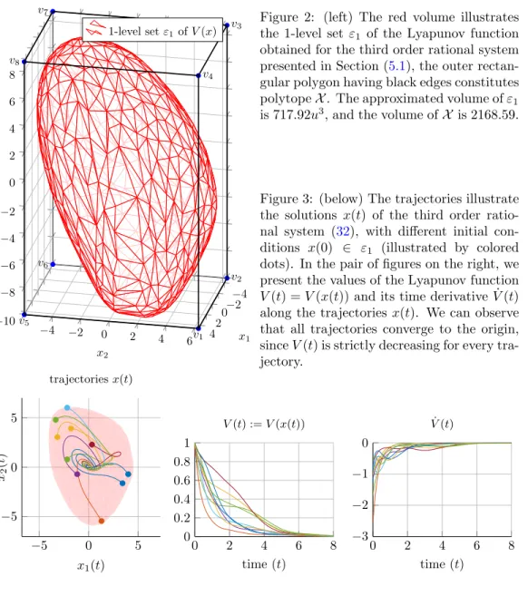
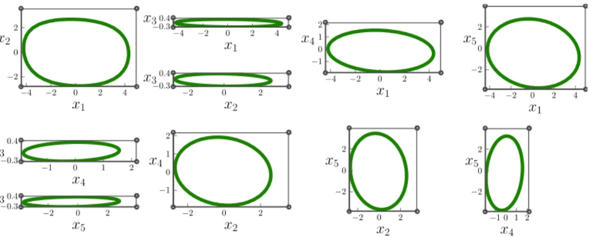
an estimate is obtained, which is illustrated in Figure 2. Furthermore, some trajectoriesx(t) are shown in Figure3from different initial conditions chosen from the inside of ε1, typically, near the edges ofε1. In the same figure, the value of the Lyapunov functionV and its time derivative ˙V can be seen along the trajectories.
The volume of the estimated DOA for the system in [1] is 32.022 cu- bic units (u3). Solving the optimization model constructed by our improved automated algorithm, the volume of the obtained invariant level set is ap- proximately 717.92u3. Polytope X was evaluated automatically using an iterative method presented in [24].
5.2. 2D uncertain Lotka-Volterra system with an uncertain positive equilib- rium point.
The system equation of ann-dimensional Lotka-Volterra (LV) model has the form
˙¯
x= diag(¯x)(A¯x+b), A∈Rn×n, b∈Rn, (34) where diag(x),x∈Rndenotes ann×nsquare diagonal matrix withx1, . . . , xn
in the main diagonal. We translate the system into its (by assumption, unique) interior equilibrium point ¯x∗ =−A−1b via introducing the centered state vectorx= ¯x−x¯∗. Then, we obtain an autonomous quasi-LPV system of the form ˙x = A(x)x, where the matrix function A can be expressed as:
A(x) = diag(x+ ¯x∗)A.
Let us consider a 2-dimensional uncertain LV system, with an uncertain model matrix A(δ) and a constant vector b, as follows:
A(δ) =
−δ1 −3 1.4 δ2
, b=
5
−2.4
, where δ1 ∈[1.8,2.2]
δ2 ∈[0.8,1.0] (35) One can immediately notice that the equilibrium point depends on the actual values of the uncertain parameters. The nontrivial equilibrium point can be given as a function of δ:
¯
x∗(δ) =ζ(δ)
7.2−5δ2
7−2.4δ1
, where ζ(δ) = 1 4.2−δ1δ2
(36) Since the value ofδ1δ2is between 1.44 and 2.2, the equilibrium point ¯x∗(δ)∈Rn is a smooth well-defined rational function of the uncertain parameters. The
−4
−2 20
−4 −2 0 2 4 6 4
−10
−8
−6
−4
−2 0 2 4 6 8
origin
v1
v2
v3
v4
v5
v6
v7
v8
x1
x2
1-level setε1ofV(x)
Figure 2: (left) The red volume illustrates the 1-level set ε1 of the Lyapunov function obtained for the third order rational system presented in Section (5.1), the outer rectan- gular polygon having black edges constitutes polytopeX. The approximated volume ofε1
is 717.92u3, and the volume ofX is 2168.59.
Figure 3: (below) The trajectories illustrate the solutions x(t) of the third order ratio- nal system (32), with different initial con- ditions x(0) ∈ ε1 (illustrated by colored dots). In the pair of figures on the right, we present the values of the Lyapunov function V(t) =V(x(t)) and its time derivative ˙V(t) along the trajectoriesx(t). We can observe that all trajectories converge to the origin, sinceV(t) is strictly decreasing for every tra- jectory.
−5 0 5
−5 0 5
x1(t) x2(t)
trajectoriesx(t)
0 2 4 6 8
0 0.2 0.4 0.6 0.8 1
time(t) V(t) :=V(x(t))
0 2 4 6 8
−3
−2
−1 0
time(t) V˙(t)
equation of the centered system is the following:
˙
x=f(x, δ) =ζ(δ) x2
1δ21δ2−4.2x21δ1+3x1x2δ1δ2−12.6x1x2+5x1δ1δ2−7.2x1δ1+15x2δ2−21.6x2
−1.4x1x2δ1δ2+5.88x1x2−3.36x1δ1+9.8x1−1x22δ1δ22+4.2x22δ2−2.4x2δ1δ2+7x2δ2
(37) We can observe that the degrees of the monomial terms in the numerators of f(x, δ) are at most 2 with respect to the elements of x. Furthermore, the monomials contain at most third order terms of the uncertain parameters, and each uncertain parameter is at most on the 2nd power. Consequently, a reasonable set of rational functions to appear in the Lyapunov function is the following:
$=n
pi(x)qj(δ)ζ(δ) pi(x)∈
x1, x2, x21, x1x2, x22 qj(δ)∈
1, δ1, δ2, δ21, δ1δ2, δ22, δ12δ2, δ1δ22 o ,
(38) which constitutes |$| = 40 rational functions. In comparison, using the LFR-toolbox, we obtained a model for which the dimension of π(0) was dim(π(0)) = 28. Finally, after the algebraic model simplification steps pre- sented in Section 3.1, we obtain a set of rational functions π, which consists of only the following 14 functions:
π=ζ(δ)
δ21δ2x21 δ1x1 δ1δ2x1 δ1δ2x1x2 δ1δ2x2 δ1δ22x22 δ1δ2x21 δ2x1 ..
δ2x2 δ2x1x2 δ22x22 δ1x21 x1x2 δ2x22T
(39) Then,Procedure1is applied to construct a maximal annihilatorNb(x, δ)∈ R25×16 for πb. The annihilator Nea of πa is given as presented in [1, Eqs.
(40,43)].
The selected set of rational functions (39) generates a parameter depen- dent Lyapunov function V(x, δ) = πbTP πb. Since the steady state also de- pends on the uncertain parameter, we compute the Lyapunov function for (34) in the original coordinates system:
V¯(¯x, δ) :=V(¯x−x¯∗(δ), δ) (40) As it is described in [1, Eq. (95)], in case of a parameter dependent Lyapunov function, we can give a lower and an upper bound for ¯V(¯x, δ) in the following way:
α1(¯x)≤V¯(¯x, δ)≤α2(¯x) for all (¯x, δ)∈Rn× D such that ¯x−x¯∗(δ)∈ X (41)
0 0.5 1 1.5 2 2.5 0
0.5 1 1.5 2 2.5
¯ x1
¯x2
εα1, area: 2.0746u2 εα2, area: 0.8631u2
¯ x∗ δ(i)
ε1 δ(j) Figure 4: The estimated DOA for sys- tem (35) is given by two regions: εα2
bounded by the closed green line and εα1
bounded by the closed red line. The closed dashed lines illustrate the 1-level set of the Lyapunov function for some partic- ular values of the uncertain parameters:
δ(i)∈ {(δ1, δ2)|δ1∈ {1.8,2,2.2}, δ2∈ {0.8,1}}. The black dots illustrate the equilibrium point of the system for certain values ofδ.
where α1, α2 : Rn → R are scalar valued positive definite proper functions, thus their 1-level set εα1 ={x¯∈Rn|α1(¯x)≤1}, εα2 = {x¯∈Rn|α2(¯x)≤1} are compact sets. These bounds should approach the Lyapunov function as much as possible, in order to obtain a larger DOA, which is described by the two level sets εα2 ⊆εα1. Even though εα2 is not invariant, we can state that any trajectory starting from an initial condition from the inside of εα2 will not leave εα1. Figure 4illustrates the estimated DOA for system (35) in the original coordinates system.
Remark 5.1. Regions εα1 and εα2 can be numerically approximated by con- sidering the union and the intersection, respectively, of the 1-level set of the Lyapunov function for discrete values of the uncertain parameters (e.g., one can consider a mesh grid on D).
The polytopeX was chosen manually to be
X = co{(−0.584,−0.4651),(1.3487,−0.433),(0.6261,0.2426) (−0.1807,−0.7064),(−0.4412,0.8298),(−0.8782,0.7172)
(1.0798,−0.7788),(1.3739,−0.5938),(−0.7941,−0.1354)} (42) where co(·) denotes the convex hull of a given set.