LINEAR ALGEBRA Lecture Notes for the Course Linear Algebra

(1)

LINEAR ALGEBRA

Lecture Notes for the Course Linear Algebra

Dorm´ an Mikl´ os, PhD

Methodological expert: Edit Gy´afr´as

(2)

Preface

This text is devoted to those students in economics who study basic linear algebra. These are short notes for the course Linear Algebra (60A105). The goal of the notes is to help students in preparing for the written tests and the exam.

We assume only minimal basic knowledge. However, knowledge of high school material is essential for understanding and learning our new concepts.

Of course, in a subject such as this, reading is not enough. Practice is also necessary, which is one of the main emphases of the book. It is about methods and their application. There are three aspects of this provided by this book:

description, solved examples and exercises. All three are important, but the most important of these is the exercises, because in mathematics you do not know a concept until you can use it.

The solved examples are integrated with the text, and the careful reader will follow the examples through at the same time as reading the descriptive material.

At the end of each chapter, exercises will help you understand the theoretical material. The range and difficulty of the tasks are quite wide. In general, solving theoretical problems is a more serious problem. The results of the calculation tasks can be found in Chapter 9. For theoretical exercises, we recommend you to consult with your lecturer/supervisor.

The relationship between the chapters can be seen in Figure 1 on the next page.

Dorm´an Mikl´os

Department of Algebra and Number Theory Bolyai Institute, University of Szeged

(5)

Section 1:

Matrices

Section 2:

Determinants

Section 3:

Linear systems

Section 4:

Vector spaces

Section 5:

Linear programming

Section 6:

Leontief model

Section 7:

Eigenvalues and eigenvectors

Section 8:

Quadratic forms

Figure 1: The relationship between the chapters

(6)

Learning Outcomes

Regarding knowledge. The student

t is familiar with the basic concepts of linear algebra;

t uses the basic vocabulary of linear algebra correctly in writing and in oral communication;

t also knows the essential methods of collecting information and the modes of statistical and mathematical analysis.

The student should be able to perform the following tasks.

Matrices (Chapter 1)

t Qualitative describe features of a matrix, e.g., diagonal, upper or lower triangular; identify special matrices like the zero matrix and the identity matrix.

t Perform matrix operations: scalar multiplication, addition and multiplication. Recognize when two matrices can be multiplied, multiply matrices.

t Define and compute the inverse of a matrix using various methods. Know and use equivalent conditions for an invertible matrix.

Determinants (Chapter 2)

t Find the determinant, minors and cofactors of a given matrix.

t Use the determinant to decide whether a given matrix is singular or nonsingular.

t Use properties of determinants.

Systems of Linear Equations (Chapter 3)

t Recognize a linear equation in nvariables.

t Find a parametric representation of a solution set of a system of linear equations.

t Write a system of linear equations in matrix form. Find the matrix and the augmented matrix of a system of linear equations.

t Solve a system of linear equations by substitution, Gaussian elimination, and Cramers Rule.

t Determine whether a system of linear equations is consistent or inconsistent.

t Find a general solution of a consistent system.

Vector Spaces (Chapter 4)

t Perform vector operations for vectors in Rⁿ.

(7)

t Recognize standard examples of vector spaces: real n-tuples (Rⁿ), the set of all m×nmatrices(R^m×n).

t Determine whether a given subset of a vector space is a subspace .

t Recognize subspaces ofR² andR³ and understand their geometric interpre- tations.

t Determine whether a vector is a linear combination of a given finite set of vectors in a vector space and be able to write this linear combination.

t Determine whether a given set of vectors in a vector space is a spanning set for that vector space.

t Determine whether a given finite set of vectors in a vector space is linearly independent.

t Determine whether a given set of vectors in a vector space forms a basis.

Recognize the standard bases in the vector spacesRⁿ and the set of all real m×n matrices(R^m×n).

t Find the dimension of a subspace inRⁿ.

t Find a basis for the column or row space of a matrix.

t Find the coordinate vector for a vector relative to a basis.

Linear programming (Chapter 5)

t Formulate a given simplified description of a suitable real-world problem as a linear programming model in general, standard and canonical forms.

t Sketch a graphical representation of a two-dimensional linear programming model given in general, standard or canonical form.

t Solve a two-dimensional linear programming problem graphically.

t Use the simplex method to solve small linear programming models by hand, given a basic feasible point.

Leontief input/output model (Chapter 6)

t Write down the consumption matrix (also called input-output matrix) of a given economy.

t Write down the matrix equation describing the necessary production levels, which would balance the given (closed or open) economy.

t Solve the appropriate equation for the given closed or open economy to find the necessary production levels of all sectors.

Eigenvalues and eigenvectors (Chapter 7)

t Verify an eigenvalue and an eigenvector of a given matrix.

(8)

t Find the characteristic polynomial and the eigenvalues and corresponding eigenvectors of a given matrix.

t Determine whether a given matrix is diagonalizable.

t Find (if possible) a nonsingular matrix P for a given matrix A such that PAP⁻¹ is diagonal.

t Find the eigenvalus of a given symmetric matrix and determine the dimension of the corresponding eigen space.

Quadratic forms (Chapter 8)

t For a real symmetric matrix write the corresponding quadratic form, and for a real quadratic form find its matrix.

t Find the type of a real quadratic form.

Regarding skills. The student

t can uncover facts and basic connections, can arrange and analyse data systematically using the structures of linear algebra;

t can make informed decisions in connection with routine and partially unfamiliar issues both in domestic and international settings;

t is capable of calculating the complex consequences of economic pro- cesses and organisational events using methods in linear algebra.

t analyze and solve problems in economics using the tools of linear algebra keeping in mind the conditions under which the methods work and the limitations of the models used;

Regarding attitude. The student

t is open to new information, professional knowledge and methodologies;

t is also open to take on task demanding responsibility in connection with both solitary and cooperative tasks;

t strives to expand his/her knowledge and to develop his/her work rela- tionships in cooperation with his/her colleagues.

t is able to work together with others in teams and projects in a con- structive, cooperative and active way;

t knows and keeps the rules and ethical norms of cooperation and lead- ership as part of a project, a team and a work organisation.

Regarding autonomy and responsibility. The student

t takes responsibility for his/her analyses, conclusions and decisions.

(9)

1 Matrices

Arthur Cayley was the first who studied systematically in a series of papers the matrices and their operations in the 19th century.

The term matrix, in mathematics, refers to any rectangular array that contains mathematical entities. In the notes, these entities will usually be real numbers. Matrices are extremely useful and fruitful mathematical structures. This section is devoted to introduce the operations for matrices and their properties.

Because of the non-commutativity of matrix multiplication this operation requires a special attention.

Topics: Matrix operations.

1.1 Matrices

Definition 1.1. A (real) matrix is a rectangular array of real numbers (in square brackets). The numbers are called the entries of the matrix. A matrix is said to be an m×n matrix or a matrix of size m×n (m, n ∈ N) if the number of rows and columns are m and n, respectively.

Example 1.2. The following object is a matrix:

1 2 3

−3 −2 √ 2

, it has two rows and three columns.

Definition 1.3. The set of allm×nmatrices with real entrieswill be denoted by R^m×n. If A ∈ R^m×n then A has m rows and n columns. The rows are numbered from the top down, and the columns are numbered from left to right.

Definition 1.4. The(i, j)-entry of the matrix A∈ R^m×n will be denoted by a_i,j or A_i,j (16i6m, 16j6n).

Example 1.5. The matrix

1 2 3

−3 −2 √ 2

has two rows and three columns;

therefore, it is a 2×3 matrix.

The (2, 3)-entry of the matrix is √

2, that is, √

2 is the third element in the second row.

Definition 1.6. The extended form of A is

A=







a1,1 a1,2 · · · a1,m

a_2,1 a_2,2 · · · a_2,m ... ... . .. ... a_n,1 a_1,2 · · · a_n,m,





 .

(10)

The matrix A has a more compact form: [a_i,j]m×n. In general, in a compact form of A the entries are described by a ‘simple’ formula.

Example 1.7. A compact form of matrix





2 5 10 17 5 8 13 20 10 13 32 25



 is (i²+j²)3×4, where the number of rows is 3, the number of columns is 4, and the i²+j² is the (i, j)-entry of the matrix is i²+j².

Definition 1.8. Two matrices A andB areequal (in written A=B) if they have the same size (say m×n) and the corresponding entries are equal, that is, equality A_i,j =B_i,j holds for every index pair (i, j), where 16i, j6n.

Example 1.9. The matrices





2 5 10 17 5 8 13 20 10 13 32 25



 and (i² +j²)3×4 are equal.

The first matrix is in extended form, while the second matrix is in compact form.

Definition 1.10. LetA∈R^m×n andB∈R^r×s be matrices. TheirsumA+B is defined if and only if A and B have the same size. If m = r and n = s then A+B∈R^m×n and

A+B=







A_1,1+B_1,1 . . . A_1,n+B_1,n ... . .. ... A_m,1+B_m,1 . . . A_m,n+B_m,n





.

Example 1.11. If A=

11 −21 7 14

, B= [ij−i+j]2×3, andC=

−11 21

−7 −13

then the sum A+B does not exist, the sum of matrices A and C exists:

A+C=

11+ (−11) −21+21 7+ (−7) 14+ (−13)

= 0 0

0 1

. Theorem 1.12. If A, B, and C are matrices of the same size then

A+B=B+A, (commutative law)

A+ (B+C) = (A+B) +C. (associative law)

Definition 1.13. A matrix is called zero matrix if all of its entries are0. A zero matrix of size m×n will be denoted by 0m×n. The negative of a matrix A is obtained from A by multiplying each entry of A by −1. The difference of matrices A and B is A−B^def.= A+ (−B).

(11)

Theorem 1.14. For every m×n matrix A we have that (a) A+0m×n =0m×n+A=A,

(b) A+ (−A) = (−A) +A=0m×n.

Definition 1.15. If A = [a_i,j]m×n is an m ×n matrix and λ is any real number then the scalar multiple λ·A of A is the m×n matrix [λa_i,j]m×n. Example 1.16. If A=

11 −21 6

7 14 −8

and λ= −3 then

λ·A=

(−3)·11 (−3)·(−21) (−3)·6 (−3)·7 (−3)·14 (−3)·(−8)

=

−33 63 −18

−21 −42 24

. Theorem 1.17. Let A be an m×n matrix and λ be a real number. Then

0·A=0m×n and λ·0m×n=0m×n.

Theorem 1.18. Let A, B, and C be arbitrary m×n matrices and λ, µ be real scalars. Then

(1) A+B=B+A,

(2) (A+B) +C= (A+B) +C, (3) A+0_m×n =0_m×n+A=A, (4) A+ (−A) = (−A) +A=0m×n, (5) λ·(A+B) =λ·A+λ·B, (6) (λ+µ)·A=λ·A+µ·A, (7) (λµ)·A=λ·(µ·A), (8) 1·A=A.

Definition 1.19. Let A be an m ×n matrix. The transpose of A is the n×m matrix whose rows are just the columns of A in the same order. The transpose of A will be denoted by A^T.

Example 1.20. If A=

11 −21 6

7 14 −8

∈R^2×3 then its transpose is

A^T =





11 7

−21 14 6 −8



∈R^3×2.

(12)

Theorem 1.21. Let Aand Bbe arbitrary m×nmatrices and λ be any real number. Then

(a) A^T is an n×m matrix, (b) (A^T)^T =A,

(c) (λ·A)^T =λ·A^T, (d) (A+B)^T =A^T +B^T.

Definition 1.22. A matrix is said to be symmetric if A^T =A.

Theorem 1.23. The matrix A ∈ R^m×n is symmetric if and only if m =n (that is,Ais a square matrix) andA_i,j=A_j,ifor all indexesi, j(16i, j6n).

Example 1.24. If A =

11 −21 7 14

and B =

11 −21

−21 15

then A is not symmetric (e.g., A_1,2 6=A_2,1), but B is symmetric.

Definition 1.25. Let A and B be matrices with A ∈ R^m×n and B ∈ R^r×s. The product of A and B is defined if and only if n=r. (To be continued) Definition 1.26. Let A and B be matrices with A ∈ R^m×n and B ∈ R^n×s. Then the product of A and B is defined, the product AB of A and B is the m×s matrix whose (i, j)-entry is computed in the following way:

Multiply each entry of row i of A by the corresponding entry of columnj of B, and add the results.

This is the dot product of row i (of A) and column j (of B).

LetA and B matrices that have sizes:

A B

m × n r × s

Their product ABis defined only ifn=r; if n=rthen ABis of sizem×s:

A B

m × n = r × s AB∈R^m×s.

(13)

Example 1.27. Let

A=

2 −3 6 3 −14 −8

, B=





2 −3

6 3

−14 −8



, and C=

2 −3 3 −14

.

Then we can form nine products with two factors with the aid of A, B, C:

A·A, A·B, A·C, B·A, B·B, B·C, C·A, C·B, C·C.

The products A·A, A·C, B·B, C·B do not exist, while the others are the following:

A·B=

2·2+ (−3)·6+6·(−14) 2·(−3) + (−3)·3+6·(−8) 3·2+ (−14)·6+ (−8)·(−14) 3·(−3) + (−14)·3+ (−8)·(−8)

=

−98 −63 34 13

, B·A=





−5 36 36 21 −60 12

−52 154 −20



,

B·C=





−5 36 21 −60

−52 154



, C·A=

−5 36 36

−36 187 130

, C·C=

−5 36

−36 187

.

Products A·B and B·A show that matrix product is not commutative:

A·B6=B·A.

Definition 1.28. Let A be anm×n matrix. The matrix A is said to be a square matrix if m=n. Themain diagonal of a square matrix of size n×n consists of the elements ai,i (i = 1, . . . , n). The identity matrix is a square matrix with 1’s on the main diagonal and0’s elsewhere. The identity matrix of size n×n will be denoted by I_n.

Theorem 1.29. Let A be an arbitrary matrix of size m×n. Then I_mA=A and AI_n =A.

(14)

Theorem 1.30 (Associative law). Let A, B, and C be matrices such that AB and (AB)C exist. Then

(AB)C=A(BC).

Example 1.31. If

A=

1 2 3 4 4 3 2 1

, B=







1 1 1

1 1 −1

1 −1 1

−1 1 1







, C=





2 2

2 −2

−2 2





then both of the products (AB)C and A(BC) exist:

(AB)C=

2 4 6 8 6 4

| {z }

AB





2 2

2 −2

−2 2



=

0 8 20 12

,

A(BC) =

1 2 3 4 4 3 2 1







2 2

6 −2

−2 6

−2 −2







| {z }

BC

=

0 8 20 12

.

Theorem 1.32 (Distributive laws). Let A, B, and C be matrices such that the indicated operations can be performed. Then

A(B+C) =AB+AC and (B+C)A=BA+CA.

Example 1.33. Let A, B and C be the following matrices:

A= 1 2

4 3

, B=

1 1 1 1 1 −1

, C=

2 2 3 2 −2 2

. Then the matrices A(B+C) and AB+AC exist, moreover,

A(B+C) = 1 2

4 3

1 1 1 1 1 −1

+

2 2 3 2 −2 2

= 1 2

4 3

3 3 4 3 −1 1

=

9 1 6 21 9 19

AB+AC= 1 2

4 3

1 1 1 1 1 −1

+

1 2 4 3

2 2 3 2 −2 2

=

3 3 −1 7 7 1

+

6 −2 7 14 2 18

=

9 1 6 21 9 19

. While, (B+C)A and BA+CA do not exist.

(15)

Theorem 1.34. Let A and B be matrices such that AB exists, and let λ be an arbitrary scalar. Then

(a) λ·(AB) = (λ·A)B=A(λ·B), (b) (AB)^T =B^TA^T.

Warning!

If the order of the factors in a product of matrices changed, the product may change (or may not exist).

Example 1.35. If A, B and C are the following matrices:

A= 0 1

1 1

, B=

1 0

−1 0

, C=

−1 0 1 1

,

then the matrices ABC, ACB, BAC, BCA, CAB and CBA are pairwise distinct 2×2 matrices:

ABC = 1 0

0 0

, ACB =

0 0

−1 0

,

BAC=

1 1

−1 −1

, BCA =

0 −1 0 1

,

CAB=

1 0

−1 0

, CBA =

0 −1 0 0

.

Remark 1.36. (a) For matrix multiplication the cancellation laws¹ do not hold, that is,

– the equality AB=AC does not imply B=C and – the equality BA=CA does not imply B=C.

(b) There are matrices A∈R^m×n andB∈R^n×p such thatAB=0m×p, but A6=0m×n and B6=0n×p.²

Definition 1.37. A square matrix is said to bediagonalif each entry outside the main diagonal is 0. A square matrix is said to be lower/upper triangular if all the entries above/below the main diagonal is 0.

1For real numbers the cancellation law states that ifab=acthenb=c(a, b, c∈R).

In this case we have only one law. Why?

2For real numbersa andbwe have thatab=0impliesa=0orb=0.

(16)

1.2 Exercises for Matrices

Exercise 1.2.1. Simplify the expressionA(BC−CD)+A(C−B)D−AB(C− D).

Exercise 1.2.2. Suppose that A, B, and C are n×n matrices and both A and B commute with C (that is, AC = CA and BC =CB). Show that AB commutes with C.

Exercise 1.2.3. Show thatAB=BAif and only if(A−B)(A+B) =A²−B². Exercise 1.2.4. Write the following system of linear equations as a single matrix equation.

3x1−2x2+x3 =4 2x₁+x₂−x₃ =7

Exercise 1.2.5. Compute the following matrix products:

1 −3 2 −2

2 −1 0 1

,

1 −1 2 2 0 4





2 3 1 1 9 7

−1 0 2



.

Exercise 1.2.6. Compute the following matrix products:



 2 1

−7





1 −1 3 ,





a 0 0 0 b 0 0 0 c









a⁰ 0 0 0 b⁰ 0 0 0 c⁰



.

Exercise 1.2.7. Given A =

1 −1 0 1

, B =

1 0 −2 3 1 0

, C =



 1 0 2 1 5 8



, and

D =

3 −1 2 1 0 5

, verify the followings: A(B−D) = AB−AD, A(BC) = (AB)C, (CD)^T =D^TC^T.

Exercise 1.2.8. Verify that A²−A−6I2=02×2 if A=

2 2 2 −1

.

Exercise 1.2.9. If A ∈ R^2×2 commutes with 0 1

0 0

then A =

a b 0 a

for some real numbers a and b.

Exercise 1.2.10. If A² can be formed, what can be said about the size ofA?

(17)

Exercise 1.2.11. Find two 2×2 matrices A such that A² =02×2.

Exercise 1.2.12. LetAandBbe symmetric matrices of the same size. Show that AB is symmetric if and only if AB=BA.

Exercise 1.2.13. Find all matrices A ∈ R^2×2 such that A^TA = AA^T (or with other words, A commutes with A^T).

Exercise 1.2.14. Show that AA^T is a symmetric matrix.

Exercise 1.2.15. Show that AB−BA=In is impossible.

Exercise 1.2.16. Let A, B, C, and D be the following matrices:

A= 2 1

0 1

, B=

1 2 −3 0 1 2

, C=





2 −1

−3 1 2 −4



, D =





0 −1 −1

−1 0 −1

−1 −1 0



. Compute the determinants of following matrices:

(a) A+B, (b) B^T −C, (c) D−2·D^T,

(d) AB, BA, (e) BC, CB, (f) DC,

(g) (A+A^T)(B+C^T), (h) DB^T, (i) BD^T, (j) A⁴, B², (k) (B+C^T)^TD, (l) D².

(In the last row, the n^th power of a matrix X is the n-fold product X· · ·X, if it exists, e.g., A⁴=AAAA and B² =BB.)

Exercise 1.2.17. A car manufacturer who produces three different models in three different plants A, B, and C reaches the production levels in million of dollars in the first and second half of the year as follows:

First half

Model 1 Model 2 Model 3

Plant A 27 44 51

Plant B 35 39 62

Plant C 33 50 47

Second half

Model 1 Model 2 Model 3

Plant A 25 42 48

Plant B 33 40 66

Plant C 35 48 50

Summarize this information in matrix form and find the total production by each plant for the whole year.

(18)

Exercise 1.2.18. Suppose thatU=

1 2 0 −1

andAU=0_2×2. Is it true that A=02×2?

Exercise 1.2.19. Let A = 1 4

5 6

. Find real numbers x, y, z, w such that A=

1 0 x 1

y z 0 w

.

Exercise 1.2.20. The matrixA is said to be idempotentif A² =A. Verify that the matrix





1/6 −1/3 1/6

−1/3 2/3 −1/3 1/6 −1/3 1/6





is idempotent. Why is it ‘good’ ?

(19)

2 Determinants

The theory of determinants was initiated by Leibnitz, in 1696.

The term ‘determinant’ occurs for the first time in Gauss’sDis- quisitiones arithmeticae(1801).

This section presents the most important properties of com- putation of determinants.

Topics:Determinants of order 2 and 3. Definition of the determinant of ordern, Laplaces formula. The basic properties of determinants; transpose, duality principle. Inverse of a matrix.

2.1 Determinants

Definition 2.1. If A = [a_1,1] is a 1 ×1 matrix then its determinant is

|A|=a_1,1. If A=

a_1,1 a_1,2 a_2,1 a_2,2

is a 2×2 matrix then its determinantis

|A|=

a_1,1 a_1,2 a2,1 a2,2

=a_1,1a_2,2−a_1,2a_2,1.

If A=





a1,1 a1,2 a1,3

a_2,1 a_2,2 a_2,3 a_3,1 a_3,2 a_3,3



 is a 3×3 matrix then its determinant is

|A|=a_1,1

a_2,2 a_2,3 a_3,2 a_3,3

−a_1,2

a_2,1 a_2,3 a_3,1 a_3,3

+a_1,3

a_2,1 a_2,2 a_3,1 a_3,2 . Example 2.2. Let A, B, and C be the following matrices:

A= 2016

, B=

1001 1055 1222 1301

, C=





1335 1458 1479 1485 1490 1605 1765 1780 1782



.

Then

|A|=2016,

|B|=1001·1301−1055·1222=13 091,

|C|=1335·

1490 1605 1780 1782

−1458·

1485 1605 1765 1782

+1479·

1485 1490 1765 1780

=22 593 540.

(20)

Definition 2.3. Let A be a matrix of size n×n (n >4). Then the determinant of A is

|A|=

a_1,1 a_1,2 · · · a_1,n a_2,1 a_2,2 · · · a_2,n ... ... ... a_n,1 a_n,2 · · · a_n,n

=a_1,1·(−1)¹⁺¹D_1,1+· · ·+a_1,n·(−1)¹⁺ⁿD_1,n, where

D1,j =

a_2,1 · · · a_2,j−1 a_2,j+1 · · · a_2,n

... ... ... ...

a_n,1 · · · a_n,j−1 a_n,j+1 · · · a_n,n is the minor of A corresponding to (1, j)-entry of A (16j6n).

LetA and Bbe square matrices of size n×n. If AB=BA=E_n then B is said to be the inverse of A.

Theorem 2.4. The square matrix A has inverse if and only if |A|6=0. If A has an inverse then the inverse is unique, and it will be denoted by A⁻¹. Theorem 2.5. Let A and B square matrices of the same size.

(a) If two rows (or columns) of a A are identical, then |A|=0.

(b) If two rows (or columns) of aA are interchanged, then only the sign of

|A| is changed.

(c) The value of |A| is unchanged if a multiple of a row is added to another row, or if a multiple of a column is added to another column.

(d) |AB|=|A|·|B|.

(e) If A is invertiblewith inverse A⁻¹, then |A⁻¹|= 1

|A|.

If A is a square matrix of size n×n with extended form A= [a_i,j]_n×n, then

(f)

a_1,1+a_1,1⁰ · · · a_1,n+a_1,n⁰

a_2,1 · · · a_2,n

... ...

a_n,1 · · · a_n,n

=

a_1,1 · · · a_1,n a_2,1 · · · a_2,n

... ...

a_n,1 · · · a_n,n

+

a_1,1⁰ · · · a_1,n⁰ a_2,1 · · · a_2,n

... ...

a_n,1 · · · a_n,n ,

(21)

(g)

λ·a_1,1 · · · λ·a_1,n

a_2,1 · · · a_2,n

... ...

a_n,1 · · · a_n,n

=λ·

a_1,1 · · · a_1,n a_2,1 · · · a_2,n

... ...

a_n,1 · · · a_n,n .

Statements (f) and (g) are true for arbitrary rows and columns.

Theorem 2.6. Let A be a square matrix. Then |A^T|=|A|.

Theorem 2.7 (Duality principle). If in a statement that is true for arbitrary determinants we interchange the words ‘row’ and ‘column’, then we get a statement that is also true for arbitrary determinants.

Definition 2.8. Let n be a natural number, A= (a_i,j) be an n×n matrix.

The minor that corresponds to the (i, j)-entry (1 6i, j 6 n) is the determinant of the (n−1)×(n−1) matrix obtained by deleting the i-th row and j-th column.

Example 2.9. Let A=





3 1 4 1 5 9 2 6 5



∈R^n×n. Then A has nine minors:

D_1,1 = 5 9

6 5

, D_1,2 = 1 9

2 5

, D_1,3 = 1 5

2 6

,

D_2,1 = 1 4

6 5

, D_2,2 = 3 4

2 5

, D_2,3 = 3 1

2 6

,

D_3,1 = 1 4

5 9

, D_3,2 = 3 4

1 9

, D_3,3 = 3 1

1 5

.

Theorem 2.10. The determinant of matrix A ∈ R^n×n can be expanded according to an arbitrary row:

|A|=a_i,1·(−1)ⁱ⁺¹D_i,1+· · ·+a_i,n·(−1)ⁱ⁺ⁿD_i,n.

Theorem 2.11. The determinant of matrix A ∈ R^n×n can be expanded according to an arbitrary column:

|A|=a_1,j·(−1)^1+jD_1,j+· · ·+a_n,j·(−1)^n+jD_n,j.

(22)

Example 2.12. Let d be the value of the determinant

1 2 1 2 1 11 1 1 3 2 1 12 1 1 1 1

. By Theorems 2.10 and 2.11 we get that

d= (−1)²⁺¹·1·

2 1 2 2 1 12 1 1 1

+ (−1)²⁺²·11·

1 1 2 3 1 12 1 1 1

+ (−1)²⁺³·1·

1 2 2 3 2 12 1 1 1

+ (−1)²⁺⁴·1·

1 2 1 3 2 1 1 1 1 (expanding by the second row),

d= (−1)¹⁺⁴·2·

1 11 1 3 2 1 1 1 1

+ (−1)²⁺⁴·1·

1 2 1 3 2 1 1 1 1

+ (−1)³⁺⁴·12·

1 2 1 1 11 1 1 1 1

+ (−1)⁴⁺⁴·1·

1 2 1 1 11 1 3 2 1

(expanding by the fourth column). The value of the determinant is 20.

(23)

2.2 Exercises for Determinants

Exercise 2.2.1. Compute the determinant of the magic square that can be seen in Figure 2.

Figure 2: A magic square in Albrecht D¨urer’s celebrated engraving of 1514 titled Melancholia I

Exercise 2.2.2. Compute the following determinants:

(a)

1 −1 0 1 1 −1

0 1 1

, (b)

1 −1 0 0 1 1 −1 0

0 1 1 −1

0 0 1 1

.

Exercise 2.2.3. Compute the following determinants:

(a)

2 −1 3 2

, (b)

6 9 8 12

, (c)

a² ab ab b² ,

(d)

cosα −sinα sinα cosα

, (e)

4 9 2 3 5 7 8 1 6

, (f)

2 0 −3 1 2 5 0 3 0

,

(g)

1 2 3 4 5 6 7 8 9

, (h)

1 b c b c 1 c 1 b ,

(i)

1 15 14 4 12 6 7 9 8 10 11 5 13 3 2 16

, (j)

1 0 −1 0 0 3 0 2 1 0 2 1 0 5 0 7 ,

(24)

(k)

1 −1 5 2

3 1 2 4

−1 −3 8 0 1 1 2 −1

, (l)

0 0 0 a 0 0 b p 0 c q k d s t u .

Exercise 2.2.4. Find real numbers x and y such that |A|=0 if:

(a) A=

0 x y y 0 x x y 0

, (b) A=

1 x x

−x −2 x

−x −x −3 ,

(c) A=

1 2 3 4 x 6 7 8 9 .

Exercise 2.2.5. Let A, B, and C be square matrices of the same size with determinants |A|= −1, |B|=2, and |C|=3. Evaluate:

(a) |A²BC^TB⁻¹|, (b) |B²C⁻¹AB⁻¹C^T|, (c) |B⁻¹AB|. Exercise 2.2.6. Solve each of the following by Cramer’s rule:

(a)

2x+y+z = 1

3x+7y−z = 5 (b)

6x+10y = 1 3x+5y = 5 (c)

7x+9y = −1

3x+4y = 5 (d)





5x+y−z = −7 2x−y−2z = 6

3x+2z = −7 (e)





4x−y+3z = 2 6x+2y−z = 3 3x+3y+2z = 5

Exercise 2.2.7. Explain what can be said about |A| if A is a square matrix of size n×n and

(a) A² =A, (b) A²=I_n,

(c) A³ =A, (d) A²+I_n =0n×n.

(25)

3 Linear systems

A linear system is a collection of linear equations. Linear systems will constitute one of the most important tool in introduc- tory linear algebra.

The section presents a systematic method for solving linear systems.

Topics: The Rouch´e-Capelli (known also as Kronecker- Capelli) theorem. Solution of the general system of linear equations. Gaussian elimination, reduction to Cramers rule. Homo- geneous system of linear equations. Solution of matrix equations.

3.1 Linear systems

Definition 3.1. A linear systemwith m equations andn variables (over the set of real numbers):











a1,1·x1+· · ·+a1,n·xn = b1, a_2,1·x₁+· · ·+a_2,n·x_n = b₂,

... a_m,1·x₁+· · ·+a_m,n·x_n = b_m.

(1)

Coefficients of the linear system: a_i,j (1 6 i 6 m, 1 6 j 6 n), variables of the linear system: x₁, . . . ,x_n, constants of the linear system: b₁, . . . ,b_m. The matrix of the linear system is

A=







a1,1 · · · a1,n

... . .. ... a_m,1 · · · a_m,n





∈R^m×n,

the augmented matrix of the linear system is

[A|b] =







a1,1 · · · a1,n b1

... . .. ... ... a_m,1 · · · a_m,n b_m





∈R^m×(n+1).

The n-tuple (c₁, . . . , c_n) is a solution the linear system if for every index i (16i6n) equality a_i,1·c₁+· · ·+a_i,n·c_n =b_i holds.

Example 3.2. The linear system

x1 + x2 − 2x3 = 5

x₁ − x₃ = 2

(26)

has the following matrix and augmented matrix:

A=

1 1 −2 1 0 −1

,

A|b

=

1 1 −2 5 1 0 −1 2

,

respectively. A particular solution is (3, 4, 1) and the general solution: (2+ t, 3+t,t) (t ∈R).

Definition 3.3. Linear system (1) is regular if m =n (that is, the matrix of the linear system is a square matrix) and the determinant

a1,1 · · · a1,n

... . .. ... a_n,1 · · · a_n,n

of the matrix of the linear system is not 0.

Example 3.4. The linear system in Example 3.2 is not regular since the matrix of the linear system is not a square matrix.

Theorem 3.5 (Cramer’s rule). If linear system (1) is regular then it has exactly one solution:

x_j =

a_1,1 · · · a_1,j−1 b₁ a_1,j+1 · · · a_1,n ... ... ... ... ... a_n,1 · · · a_n,j−1 b_n a_n,j+1 · · · a_n,n

a1,1 · · · a1,j−1 a1,j a1,j+1 · · · a1,n

... ... ... ... ... an,1 · · · an,j−1 an,j an,j+1 · · · an,n

(16j6n).

Example 3.6. The linear system









3x₁+2x₂+2x₃−2x₄ = 2 2x₁+3x₂−2x₃+2x₄ = 0 2x₁−2x₂+3x₃+2x₄ = 1

−2x₁+2x₂+2x₃+3x₄ = 9

is regular since the number of variables coincides with the number of equations and the determinant

3 2 2 −2

2 3 −2 2

2 −2 3 2

−2 2 2 3

= −375

(27)

is not 0. The linear system has exactly one solution:

x₁ =

2 2 2 −2

0 3 −2 2 1 −2 3 2

9 2 2 3

3 2 2 −2

2 3 −2 2

2 −2 3 2

−2 2 2 3

= −14

15, x₂=

3 2 2 −2 2 0 −2 2

2 1 3 2

−2 9 2 3

3 2 2 −2

2 3 −2 2

2 −2 3 2

−2 2 2 3

= 4 3,

x₃ =

3 2 2 −2

2 3 0 2

2 −2 1 2

−2 2 9 3

3 2 2 −2

2 3 −2 2

2 −2 3 2

−2 2 2 3

= 23

15, x₄=

3 2 2 2

2 3 −2 0 2 −2 3 1

−2 2 2 9

3 2 2 −2

2 3 −2 2

2 −2 3 2

−2 2 2 3

= 7 15.

Definition 3.7. Elementary operations for linear systems:

• interchange two equations,

• multiply an equation by a nonzero number,

• add a multiple of an equation to another equation.

Elementary operations for matrices (only for rows):

• interchange two rows,

• multiply a row by a nonzero number,

• add a multiple of a row to another row.

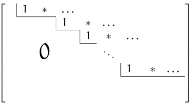
Definition 3.8. If A is a zero matrix (that is, every entry of A is zero) then it is in row-reduced or row-echelon form. A matrix A that is not a zero matrix is in row-reduced or row-echelon form if A is of the form that can be seen in Figure 3 (every entry under the broken line is 0, the starred entries (∗) may have any value). That is, a nonzero matrix is row-reduced if the following properties hold for A:

• all nonzero rows are above any rows of all zeros,

(28)







1 ∗ . . .

1 ∗ . . . 1 ∗ . . .

0

^{. ..}

1 ∗ . . .







Figure 3: A row-reduced form matrix

• each leading entry of a row is in a column to the right of the leading entry of the row above it,

• all entries in a column below a leading entry are zeros.

If Ahas the following additional two properties then it isrow-reduced echelon form:

• the leading entry in each nonzero row is 1,

• each leading 1 is the only nonzero entry in its column.

Example 3.9. The following matrices are in row-reduced form:





∗ ∗ ∗

0 0 ∗

0 0 0



,







0 ∗ ∗ ∗ ∗

0 0 0 ∗ ∗

0 0 0 0 ∗

0 0 0 0 0 0





 .

(The black squares denote non-zero elements, the starred entries (∗) may have any value.) The following matrices are in row-reduced echelon form:





1 ∗ 0 0 0 0 1 0 0 0 0 1



,







0 1 ∗ 0 0 ∗ 0 0 0 1 0 ∗ 0 0 0 0 1 ∗ 0 0 0 0 0 0





 .

(The starred entries (∗) may have any value.)

Theorem 3.10. Each matrix is row equivalent to a unique row-reduced echelon form, that is, for every matrix A there is a unique matrix B such that

(29)

• matrix B is in row-reduced echelon form,

• B can be got by elementary row operations from A.

Example 3.11. Find the row-reduced echelon form ofA=





3 3 4 3 4 3 4 3 4 3 2 6 6 8 8



.

The process can be the following:

A

1 2·row3

−→





3 3 4 3 4 3 4 3 4 3 1 3 3 4 4





row1↔row3

−→





1 3 3 4 4 3 4 3 4 3 3 3 4 3 4





(−3)·row1+row2

−→





1 3 3 4 4

0 −5 −6 −8 −9

3 3 4 3 4





(−3)·row1+row3

−→





1 3 3 4 4

0 −5 −6 −8 −9 0 −6 −5 −9 −8





(−1)·row3+row2

−→





1 3 3 4 4

0 1 −1 1 −1

0 −6 −5 −9 −8





6·row2+row3

−→





1 3 3 4 4

0 1 −1 1 −1

0 0 −11 −3 −14



.

The last matrix in the above series of matrices is a row-reduced form of A, that is,





1 3 3 4 4

0 1 −1 1 −1

0 0 −11 −3 −14



 in row-reduced form and it is equivalent to

(30)

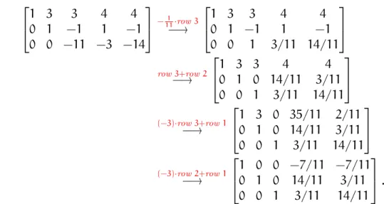
A. To get the row-reduced echelon form, we need some more steps:





1 3 3 4 4

0 1 −1 1 −1

0 0 −11 −3 −14





−₁₁¹·row3

−→





1 3 3 4 4

0 1 −1 1 −1

0 0 1 3/11 14/11





row3+row2

−→





1 3 3 4 4

0 1 0 14/11 3/11 0 0 1 3/11 14/11





(−3)·row3+row1

−→





1 3 0 35/11 2/11 0 1 0 14/11 3/11 0 0 1 3/11 14/11





(−3)·row2+row1

−→





1 0 0 −7/11 −7/11 0 1 0 14/11 3/11 0 0 1 3/11 14/11



.

Theorem 3.12. (a) If the row-reduced form of the augmented matrix of a linear system has the form in Figure 4, then the linear system has no solutions.







1 ∗ . . . b₁⁰

1 ∗ . . . b₂⁰

1 ∗ . . . b₃⁰

0

^{. ..} ^..^.

1 ∗ . . . b_k⁰ 1 0 ... 0







Figure 4: Linear system without solution

(b) If the row-reduced form of the augmented matrix of a linear system has the form in Figure 5, where b_k⁰ 6=0, then the linear system has either exactly one solution or infinitely many solutions.

(31)







1 ∗ . . . b₁⁰

1 ∗ . . . b₂⁰

1 ∗ . . . b₃⁰

0

^{. ..} ^..^.

1 ∗ . . . b_k⁰ 0

... 0







Figure 5: Linear system with non-empty solution set

Example 3.13. Compare the following two linear systems:





x₁ + 2x₂ + 3x₃ + 4x₄ + 5x₅ = 2, 3x1 + 4x2 + 3x3 + 4x4 + 3x5 = 2,

−7x₁ − 8x₂ − 3x₃ − 4x₄ + x₅ = −2,

(2)





x₁ + 2x₂ + 3x₃ + 4x₄ + 5x₅ = 2, 3x1 + 4x2 + 3x3 + 4x4 + 3x5 = 2,

−7x₁ − 8x₂ − 3x₃ − 4x₄ + x₅ = −1.

(3)

The augmented matrices of the linear systems (2) and (3) are





1 2 3 4 5 2

3 4 3 4 3 2

−7 −8 −3 −4 1 −2



,





1 2 3 4 5 2

3 4 3 4 3 2

−7 −8 −3 −4 1 −1



, respectively. Their row-reduced echelon forms are





1 0 −3 −4 −7 −2

0 1 3 4 6 2

0 0 0 0 0 0



,





1 0 −3 −4 −7 0

0 1 3 4 6 0

0 0 0 0 0 1



, respectively, which shows that the linear system (3) has no solution and linear system (2) has infinitely many solutions:

x1= −2+3x3+4x4+7x5, x₂=2−x₃−4x₄−6x₅, where x₃, x₄, x₅ are arbitrary real numbers.

(32)

3.2 Exercises for Linear systems

Exercise 3.2.1. Write a linear system of linear equations that has each of the following augmented matrices:

(a)





1 −1 6 0

0 1 0 3

2 −1 0 1



, (b)





2 −1 0 −1

−3 2 1 0

0 1 1 3



.

Exercise 3.2.2. In each case, assume that the augmented matrix of a linear system has been carried to the given row-reduced matrix by elementary row operations. Solve the linear systems.

(a)





1 0 0 −1

0 1 0 3

0 0 1 2



, (b)





1 3 0 1 −3 0

0 0 1 2 5 0

0 0 0 0 0 1



.

Exercise 3.2.3. Solve each of the following linear systems.

(a)

2x+y+z = 1

3x+7y−z = 5 (b)

x+y+z = 3 2x+y+3z = 1 (c)





3x+4y+z = 1 2x+3y = 0 4x+3y−z = −2

(d)

2x+3y+z = 5 5x+7y+z = 6

(e)





2x+5y+9z+3z = −1 x+2y+4z = 1 3x+3y+2z = 5 (f)





x−y+z = 2 x−z = 1 y+2x = 0

(g)





x+y = 1 y+z = 0 z−x = 2

(h)









2x+5y+9z+3z = 1

−x+2y+4z = 1 x+y+z+w = 1 x−y+2z+2w = 5

(33)

4 Vector spaces

Vector spaces are among the most important structures in mathematics. Although the set of axioms of vector spaces seem rather difficult, they provides a comfortable framework for our activity.

Topics: Vector spaces. Linear dependence and indepen- dence. Rank of a family of vectors, basis and dimension of a vector space. Ranks of a matrix, the row, column and deter- minantal ranks are equal. The rank and the determinant of a product of matrices. Homogeneous system of linear equations.

The subspace of solutions, fundamental systems.

4.1 Introduction to vector spaces

Definition 4.1. A real vector space is a nonempty set V (its elements will be called vectors) with a binary operation + (addition of vectors) and for each real number λ a unary operation λ· (multiplication by scalar λ, in this context, the real numbers will be called scalars) that satisfy the following eight properties for all vectors u, v, w∈V and for all scalars α, β∈R:

(1) (u⊕v)⊕w=u⊕(v⊕w), (2) v⊕0=0⊕v=v,

(3) v⊕(−v) = (−v)⊕v=0, (4) u⊕v=v⊕u,

(5) α(u⊕v) =αu⊕αv, (6) (α+β)v=αv⊕βv, (7) (αβ)v=α(βv), (8) 1v=v.

Example 4.2. Let V = R³ =







 a b c



:a, b, c∈R



 (the set of vectors), ⊕ (addition of vectors):



 a b c



⊕



 a⁰ b⁰ c⁰



=



 a+a⁰ b+b⁰ c+c⁰



 (a, b, c, a⁰, b⁰, c⁰ ∈R),

(34)

λ (multiplication by the scalar λ(∈R)):

α



 a b c



=



 αa αb αc



 (a, b, c∈R, λ∈R).

The set V with these operations constitutes a vector space, where 0 =



 0 0 0





is the zero vector and the opposite vector of v=



 a b c



∈V is −v=





−a

−b

−c



 =

(−1)



 a b c



.

Example 4.3. We can generalize the previous example. Let V =Rⁿ=

[a₁, . . . , a_n]^T :a₁, . . . , a_n ∈R ,

• addition of vectors: [a₁, . . . , a_n]^T ⊕[b₁, . . . , b_n]^T = [a₁+b₁, . . . , a_n + b_n]^T;

• multiplication by scalars: λ[a1, . . . , an]^T = [λa1, . . . , λan]^T. Then V is a vector space with these operations.

Theorem 4.4. Let V be a real vector space (that is, V is a vector space over the field R), v∈V, λ∈K. Then

(a) λv=0 if and only if λ=0 or v=0;

(b) −v= (−1)v.

Definition 4.5. Let V be a real vector space. The linear combination of vectors v₁, . . . , v_k∈V by scalars λ₁, . . . , λ_k∈R is the vector

λ₁·v₁+· · ·+λ_k·v_k. The linear combination is trivialif λ₁ =· · ·=λ_k=0.

Example 4.6. Let V = R⁴, v1 = [1, 1,−1,−1]^T, v2 = [2,−2,−2, 2]^T, and v₃ = [−3,−3, 3, 3]^T. The linear combination of vectors v₁, v₂, v₃ by scalars λ₁ =1, λ₂= −2, λ₃=3 is

λ₁·v₁+λ₂·v₂+λ₃·v₃

=1·[1, 1,−1,−1]^T +(−2)·[2,−2,−2, 2]^T +3·[−3,−3, 3, 3]^T

=[1, 1,−1,−1]^T +[−4, 4, 4,−4]^T +[−9,−9, 9, 9]^T

= [−12,−4, 12, 4]^T.

(35)

Definition 4.7. Let V be a real vector space. The vectorsv₁, . . . , v_k ∈V are said to be linearly dependentif there are scalars λ₁, . . . , λ_k ∈Rsuch that not all of them are zero and

λ₁·v₁+· · ·+λ_k·v_k=0,

that is, there is a nontrivial linear combination of vectors v₁, . . . , v_n that yields the zero vector.

Example 4.8. The vectors v₁ = [1, 2, 1]^T, v₂ = [−1,−1, 2]^T, v₃ = [5, 7,−4]^T are linearly dependent because2·v₁+ (−3)·v₂+ (−1)·v₃ is a nontrivial linear combinations of the vectors v₁, v₂, v₃ and

2·v₁+ (−3)·v₂+ (−1)·v₃ =0.

Definition 4.9. Let V be a real vector space. The vectorsv1, . . . , vk ∈V are said to be linearly independent if they are not linearly dependent.

Example 4.10. (a) The vectors

e_i = [0, . . . , 0,

i-th component

z}|{1 , 0, . . . , 0]^T (16i 6n)

are linearly independent in the real vector space V =Rⁿ, because λ₁·e₁+· · ·+λ_n·e_n = [λ₁, . . . , λ_n]^T

implies that λ₁·e₁+· · ·+λ_n·e_n =0 if and only ifλ₁ =· · ·=λ_n=0.

(b) The vectors u = [1, 2, 3, 1]^T, v = [0, 1, 1, 1]^T, w = [−1, 1, 1, 2]^T are linearly independent since for arbitrary scalars α, β, γ ∈ R we have that

α·u+β·v+γ·w=0⇐⇒







α−γ 2α+β+γ 3α+β+γ α+β+2γ







=





 0 0 0 0







⇐⇒









α−γ = 0 2α+β+γ = 0 3α+β+γ = 0 α+β+2γ = 0

⇐⇒α=β=γ=0.

(36)

4.2 Subspaces

Definition 4.11. Let V be a real vector space. The subset W of V is a subspace of V if

• 0∈W (the zero vector of V belongs to W),

• if u, u⁰ ∈W then u+u⁰ ∈W (W is closed under addition of vectors),

• if u∈ W and λ∈ R then λ·u ∈W (W is closed under scalar multiplication).

Example 4.12. • U₁ =

[x, y]^T :x+y=1 is not a subspace in R².

• U₂ =

[x, y, z]^T :x+y=z, 2x−y=3z is a subspace in R³.

Definition 4.13. Let v₁, . . . , v_n be vectors in a real vector space V. The subspace generated by the vectors v1, . . . , vn is

{α₁·v₁+· · ·+α_n·v_n :α₁, . . . , α_n ∈R},

that is, the set of all linear combinations ofv1, . . . , vn. This set will be denoted by Span(v₁, . . . , v_n).

Theorem 4.14. Let v₁, . . . , v_n be vectors in a real vector space V. Then Span(v₁, . . . , v_n) is indeed a subspace in V.

Definition 4.15. The vector system v₁, . . . , v_k in V is said to be agenerator system of the vector space V if Span(v₁, . . . , vk) =V.

A linearly independent generator system in V is called a basis.

Example 4.16. If V =Rⁿ then the vector system e₁ = [1, 0, 0, . . . , 0, 0]^T, e₂ = [0, 1, 0, . . . , 0, 0]^T,

...

e_n = [0, 0, 0, . . . , 0, 1]^T is a basis in V, this is the standard basis of V.

Example 4.17. If V =R³ then the vector system v₁ = [5, 7,−1]^T, v₂ = [4,−1, 7]^T, v₃ = [−3, 5, 2]^T

(37)

is a basis in V. The vector [3, 1, 4]^T can expressed as a linear combination of basis vectors for both bases:

[3, 1, 4]^T = [3, 0, 0]^T + [0, 1, 0]^T + [0, 0, 4]^T =3·e₁+1·e₂+4·e₃, [3, 1, 4]^T = 8

45 ·v₁+26

45 ·v₂+ 1 15 ·v₃.

Definition 4.18. A basis of a vector space is a linearly independent and generating family of vectors. A vector space is finitely generated if it has a finite set of generators.

Proposition 4.19. If F : f1, . . . , fn is a basis in V then for each vector v ∈ V there are uniquely determined scalars α₁, . . . , α_n ∈ R such that v = α₁·f₁+· · ·+α_n·f_n.

Definition 4.20. Using the notations of the previous proposition, the coordinate vector of v with respect to the basis v is [α₁, . . . , α_n]^T ∈ Rⁿ that will be denoted by [v]F.

Example 4.21. In R³ the standard basis is a basis. The vectors [5, 7,−1]^T, [4,−1, 7]^T, [−3, 5, 2]^T constitute a basis in R³, as well.

Theorem 4.22. If u₁, . . . , u_k is a generating system v₁, . . . , v_n is a basis in a finitely generated vector space, then n6k.

Theorem 4.23. In a finitely generated vector space V any two bases have the same number of elements.

Definition 4.24. The common number of elements in all bases of a finitely generated vector space V is called the dimension of V, and is denoted by dim(V).

Example 4.25. The real vector space V =Rⁿ has dimension n.

Definition 4.26. The rank of vectors v₁, . . . , v_k in a finitely generated vector space V is the dimension of Span(v1, . . . , vk), that is, rank(v1, . . . , vk) = dim(Span(v₁, . . . , v_k)).

Example 4.27. Let V be a real vector space, v, v⁰, v⁰⁰, . . .∈V. Then

• the family v is linearly independent if and only if v6=0,

• the family v, v⁰ is linearly independent if and only if v 6= 0 and v⁰ 6∈

Span(v),