hjic.mk.uni-pannon.hu DOI: 10.33927/hjic-2019-11
COMPARISON OF THE APPROXIMATION METHODS FOR TIME-DELAY SYSTEMS: APPLICATION TO MULTI-AGENT SYSTEMS
ÁRONFEHÉR*1,2ANDLORINC˝ MÁRTON1
1Department of Electrical Engineering, Sapientia Hungarian University of Transylvania, C.1., Târgu Mure¸s, 547367, ROMANIA
2Department of Mathematics, University of Pannonia, Egyetem u. 10, Veszprém, 8200, HUNGARY
This paper presents a review of dominant pole and model-approximation algorithms for delayed systems that can be applied to multi-agent systems. A novel algorithm is proposed to determine an approximation method for multi-agent systems in the platoon configuration with a communication delay. Simulations are presented to show the applicability of the proposed algorithm.
Keywords: time delay, differential equations, asymptotic properties, multi-agent systems
1. Introduction
A Multi-Agent System (MAS) consists of multiple ac- tive agents (e.g. vehicles), passive agents (e.g. obstacles), in addition to cognitive agents and their environment [1].
Every active agent is at least partially autonomous and uses a distributed control algorithm [2]. The agents can communicate with each other. This communication struc- ture is defined by a graph, where each vertex corresponds to one agent and each edge to a communication direction.
A platoon is a special MAS configuration, with a linear communication graph. The leading (first) agent implements a reference tracking algorithm. Every other agent implements a consensus with the adjacent agents [3].
With the increase in the number of agents and the physical distance between the agents, the communication delay cannot be neglected. While the stability of such sys- tems is ensured by the consensus protocol [4], the delay will influence the transient behavior of the MAS [5].
The goal of this paper is to compare the existing ap- proximation methods for the transient behavior analysis of MAS with communication delays and present a novel analysis method which can be applied to any MAS sys- tem which satisfies a smallness delay condition.
2. Modelling of MAS
A MAS is considered with agents that exhibit single- integrator dynamics [6]. The state-space model of an agent becomesx˙i(t) = ui(t), where xi ∈ R denotes
*Correspondence:fehera@ms.sapientia.ro
the state of theith agent andui∈Rrepresents the input, i= 1,2, . . . , n.
A MAS has an underlying communication graph, in which the vertex is an agent and the edge a communica- tion path [7], so the agentith in the system is the vertex vi. LetNi be the set of neighbors ofvi, so thatNi con- tains all vertices that are connected tovi.
Consensus algorithm The consensus problem of a MAS is the procedure of gathering every state from the initial condition to a common steady-state. If the commu- nication graph is connected, the consensus with regard to an agent can be reached with the input (consensus proto- col)
ui(t) = X
j∈Ni
(xj(t)−xi(t)). (1)
The adjacency matrixA= (aij)∈Rn×nof a graph with nnodes is defined as
aij :=
(1, ifi6=jandviare adjacent tovj
0, otherwise . (2)
The degree matrixD= (dij)∈Rn×nof a graph withn nodes shows the number of neighbors for each vertex and can be defined as
dij:=
(deg(vi), ifi=j
0, otherwise, (3)
wheredeg(vi)denotes the degree or the number of edges incident to vertexi.
Figure 1:The communication topology of a vehicle pla- toon system consisting ofn vehicles with time delayτ in the communication graph. The dashed line symbolizes more nodes in between, while the dotted line represents the reference input of the nodes.
With this notation the dynamics of the MAS with the consensus protocol is given by
˙
x(t) =−Lx(t), x(0) =x0, (4) whereLdenotes the Laplacian matrix [8] which is con- structed as L = D −A, D stands for the degree ma- trix, A represents the adjacency matrix of the graph, x = x1 x2 . . . xn
>
∈ Rn denotes the state vec- tor consisting of thenstates of the MAS, andx0∈Rnis a constant vector of the initial states.
According to [9] the eigenvalues of a MAS consisting ofn agents with a connected communication graph can be ordered as
0 =λ1> λ2≥ · · · ≥λn. (5) The steady states (equilibria) of the MASxssare the el- ements of the null space ofL. Given, according to the definition of the Laplacian matrix, P
j∈Nilij = 0 [6]
for every solution x of (Eq. 4): lim
t→∞x(t) = xss =
1 n
Pn
i=1xi(0)1, where1= 1 1 . . . 1>
∈Rn. MAS with delayed communication In the case of de- layed communication, the consensus protocol is of the form
ui(t) = X
j∈Ni
(xj(t−τ)−xi(t)), (6) whereτ ≥0denotes the constant communication delay which is present among adjacent agents.
According toRefs.[4] and [10], the MAS with com- munication delay (also referred to as Multi-Agent System with Delays (DMAS)) is
˙
x(t) =−Dx(t) +Ax(t−τ) +R, (7) x(θ) =x0∈Rn, θ∈[−τ,0],
3. Platoon of vehicles
A platoon of vehicles is a special class of MAS with a communication topology shown inFig. 1. The kinematic model of a vehicle can be written as
˙
xi(t) =ui(t), (8)
wherexi(t)denotes the position of the vehicle andui(t) represents the control signal in the form
(u1(t)=kp1(r−x1(t))
ui(t)=ξi(xi−1(t−τ)−d−xi(t)),∀i= 2, ..., n (9) wherei∈(1, n),n∈N, n >1,ddenotes the prescribed inter-vehicle distance,ξi >0, andkpi > 0are constant control gains.ris the position reference of the first vehi- cle.
Eqs. 8and9can be written as a system of differential equations with delay:
˙
x(t) =−Φx(t) + Γx(t−τ) +f
1r−f
2d, (10) where
Φ = diag{ kp1 ξ2 . . . ξn−1 ξn
} (11) denotes the degree matrix with the state feedback,
Γ =
0 0 0 . . . 0 0 0
ξ2 0 0 . . . 0 0 0 ... ... ... . .. ... ... ... 0 0 0 . . . ξn−1 0 0 0 0 0 . . . 0 ξn 0
(12)
represents the adjacency matrix, and f1= kp1 0 . . . 0>
, (13)
f2= 0 ξ2 . . . (n−1)ξn>
. (14)
The homogeneous part of the relation in Eq. 10is of the same form as the relation in Eq. 7, and the term f1r−f
2drepresents the reference as well as inter-vehicle distance induced inflows.
4. Existing methods for the approximation of time-delay systems
In this section, the various current approximation meth- ods for time-delay systems are reviewed. The form of the studied systems is shown by the following relation:
˙
x(t) =−Φx(t) + Γx(t−τ), x(h) =x0, (15) which is the homogeneous part of Eq. 10, where θ(h) denotes the initial condition withh∈ [−τ,0], and has a quasi-polynomial characteristic equation:
λIn+ Φ−Γe−τ λ= 0, (16) where the delay component induces an exponential term.
The roots ofEq. 16determine the transient behaviour of the system inEq. 15. AsEq. 15possesses an infinite number of solutions, it is important to develop such an equivalent system which has a finite number of eigenval- ues and is a good approximation of the original system in Eq. 15. If a good delay-free approximation is available, it
could be applied to the transient behaviour analysis and control design for delayed systems.
Let a special solution be denoted by x, which is˜ uniquely determined by the valuex(0), and independent˜ ofθ(h), h∈[−τ,0), thus forming annparameter fam- ily. In a linear autonomous system, this corresponds to the eigensolution generated by exactly n characteristic roots (multiplicities included) which lies in the half-plane Reλ >−1/τ, seeRef.[11].
Theorem 1. [11]Consider a Delay Differential Equation (DDE) system of the form shown in relationEq. 15with a Lipschitz criterion of:
(kΦk+kΓk)τ e <1, (17) further noted assmallness condition, for every solution xofEq. 15a globally defined solution˜x:R→Rnexists that satisfies the growth conditionsupt≤0kx(t)ke˜ t/τ <
∞such that
kx(t)−x(t)k →˜ 0 exponentially ast→ ∞.
For further related discussions, seeRefs.[12] and [13].
The aforementioned theorem yieldsndominant eigenval- ues which can accurately represent a DDE system. The system shown in the relation inEq. 15uses the consensus protocol, which ensures that the eigenvalues are located in the left half-plane in the complex region. The final lo- cation of the dominant eigenvalues is created as a semi- circle with origin0, radius1/τ, and a negative real part.
4.1 The modified chain approximation
The modified chain approximation method creates an ap- proximating system directly from the state-space repre- sentation of the delayed system [14]. For a DDE in the form ofEq. 15, the modified chain approximation method yields an approximating linear system in the form of
˙
y0(t) =−Φy
0(t) +m τIny
m(t)
˙
y1(t) = Γy
0(t)−m τIny
1(t) (18)
...
˙
yk(t) = m τ Iny
k−1(t)−m
τInyk(t), 2≤k≤m The output vectorz =y
0 represents the approximation of the solutionxof the relation inEq. 15. The approxi- mating system in the form of a matrix is shown in
˙
y(t) =Gy(t) (19)
with
G=
−Φ 0n 0n · · · 0n m τIn
Γ −mτIn 0n · · · 0n 0n
0n m
τIn −mτIn · · · 0n 0n
... ... ... . .. ... ...
0n 0n 0n · · · mτIn −mτIn
(20) where y ∈ Rmn denotes the state vector, G ∈ R(m+1)n×(m+1)n represents the matrices of the system, 0n ∈ Rn×n stands for the zero matrix,nis the number of agents andm denotes the number of approximating equations.
According toRef.[14] the output of the system (Eq.
19) defined asz(t) = y
0(t)linearly converges into the solution of the original DDE system such thatc >0and supt≥0kx(t)−z(t)k ≤ mc.
4.2 The Lambert W function
The LambertW function can be used to find the domi- nant eigenvalues of a quasi-polynomial equation (Eq. 16).
EveryW(s)function that satisfies
W(s)eW(s)=s (21)
by definition is referred to as a LambertWfunction [15], wheresis either a scalar or matrix complex number func- tion. The LambertW function has multiple branches de- noted asWk(s)withk= 0,±1,±2, . . . ,±∞.
Example 4.1. If a scalar DDE is present in the form of
˙
x(t) =ax(t) +bx(t−τ) +cu(t), (22) witha, b, c, θ ∈ R, x(h) = θ(h)for h ∈ [−τ,0], the quasi-polynomial of the homogeneous part can be written as
(λ−a)eτ λ=b. (23) If both sides are multiplied byτe−aτ, then
(λ−a)τeτ(λ−a)=bτe−aτ, (24) which satisfiesEq. 21withW(bτe−aτ) = (λ−a)τ, and the eigenvalues can be calculated using the branches of the LambertW function as
λk= 1
τWk(bτe−aτ) +a. (25) In our case, in terms of the relation in Eq. 15, the aforementioned solution is generalized as
λk = 1
τWk(Γτ Qk)−Φ, (26)
whereQkcan be calculated by solving the equation nu- merically
Wk(Γτ Qk)eWk(Γτ Qk)−Φτ = Γτ (27) forQk[16].
Although many numerical solvers provide native sup- port for the solution of the scalar LambertW function, the general case requires additional solver tools. There- fore, the LambertWDDE Toolbox [17] was created. The functionfind_Skassumesτ,Γand−Φ. The returned val- ues are the eigenvaluesλk and theQk parameters for a givenkbranch. The toolbox can create the approximat- ing solution for the given system as
˜ x(t) =
m2
X
k=m1
eλktCkI, (28)
wherex˜is the approximating solution of the original de- lay system and the parameterCkI can be computed with the help offind_CIfor a givenm1< k < m2branch. In the scalar case,CkI takes the form of
CkI = x0+be−λkτRτ
0 θ(t−τ)dt
1 +bτe−λkτ . (29)
4.3 The Quasi-polynomial root-finder algo-
rithm
The quasi-polynomial root-finder algorithm calculates the dominant eigenvalues of a system based directly on the quasi-polynomial equation inEq. 16.
The quasi-polynomial equation of the system in Eq.
16can be written as:
P(λ) =
N
X
k=0
Qk(λ)e−αkτ λ, (30)
whereQkis a polynomial with real coefficients andαk ∈ R. The objective is to compute the spectrum in the region of the complex planeD ⊂ Cwith boundariesβmin <
Re(D)< βmaxandωmin<Im(D)< ωmax.
Let the surfaces defined by the real and imaginary parts ofP(λ)be:
Re(P(β, ω)) = 0 (31) Im(P(β, ω)) = 0 (32) The eigenvalues can be located at the points of in- tersection of the zero-level curves of the surfaces Re(P(β, ω)) = 0 andIm(P(β, ω)) = 0 as shown in Ref.[18]. The accuracy of the algorithm is increased by Newton’s method and by adapting the grid density ofD as shown inRef.[16].
The Quasi-polynomial root-finder algorithm (QPmR) [19] is implemented in MATLAB. The function expects the region of interest[βmin, βmax, ωmin, ωmax] to be in the complex plane of the polynomial coefficient matrix of the quasi-polynomial where one row corresponds to
one polynomial multiplied by the same exponential term.
The delay vector, computational accuracy and grid step are also required.
In our case this translates into a region of interest [−1τ,0,−τ1,τ1]if the smallness condition (Eq. 17) is sat- isfied. The first row of the matrix of polynomial coeffi- cients contains the coefficients of the delay-free part so that the delay vector is of the form[0, τ,2τ, ...].
The algorithm covers the given region with a mesh grid, then evaluates the quasi-polynomial at each point of the grid by splitting it into a real and an imaginary part.
The zero-level curves are then mapped with the help of thecontour plotting algorithm. The computational error is checked and if it is too large, the algorithm is restarted using a modified grid density as described inRef. [16].
If the computational error is smaller than the given level of tolerance, the computed dominant eigenvalues are re- turned.
5. Explicit matrix approximation method
An approximation method was devised where the con- vergence rate is exponential, the degree of the resulting system in the form ofEq. 4matches exactly the degree of the delayed MAS given inEq. 15, and the same properties are exhibited in specific cases.The Banach fixed-point theorem was used as dis- cussed inRef. [20] to explicitly find a linear system of the form ofEq. 4which approximates the homogeneous part of the system inEq. 10.
If an(X, f)metric space is present andT :B →B is a contraction with a bounded setB ⊂ X, andq < 1 such that
f(T(x), T(y))≤qf(x, y) (33) by definition T admits a unique fixed point x˜ such as T(˜x) = ˜x, and this fixed point can be found by starting from an arbitrary elementx0∈Bwith the sequence
xn =T(xn−1), (34) wherexn→x.˜
A DDE system is defined in Eq. 15 by the corre- sponding smallness condition ofEq. 16. Since all normed spaces are metric spaces, the metric spaceX =Rn×nis set withf as the induced matrix norm. The contraction T :B →Bis present such that
T(Λ) =−Φ + Γe−Λτ, (35) andB ={Λ∈Rn×n|kΛk ≤(kΦk+kΓk)e}. The rela- tion inEq. 33holds true for(kΦk+kΓk)τe<1.
LetΛ1,Λ2∈Bsuch thatkΛ1k>kΛ2k. The left side of the inequality inEq. 33can be written as
kT(Λ1)−T(Λ2)k=kΓkke−Λ1τ−e−Λ1τk.
It is evident that kΓk ≤ kΓk+kΦk and the maximum norm can be used as
ke−Λ1τ−e−Λ1τk ≤τkΛ1−Λ2keτmax{kΛ1k,kΛ2|}.
It can be seen that
kT(Λ1)−T(Λ2)k ≤τkΛ1−Λ2k(kΓk+kΦk)eτ(kΓk+kΦk)e
and by applying the smallness conditionkΓk+kΦk ≤ 1/(τe)(Eq. 17),
kT(Λ1)−T(Λ2)k ≤ kΛ1−Λ2k
is obtained, which proves thatT : B → Bis a contrac- tion. This shows that by solving
Λ =−Φ + Γe−Λτ (36) for theΛmatrix, a system is created
d˜x
dt = Λ˜x, (37)
which approximates the DDE system ofEq. 15. As a re- sult of the proposed iterative method, the eigenvalues and eigenvectors ofEq. 37approximate, with a given degree of precision, the dominant eigenvalues ofEq. 14.
5.1 Comparison with the existing methods
• Chain approximation:
+ The result is an approximating system with known system matrices (both eigenvalues and eigenvectors are known).
- The resulting system is of a higher degree than the delay system.
- The convergence rate of the algorithm is linear.
• LambertW function:
+ The result is a trajectory approximation.
+ The convergence rate of the algorithm is expo- nential.
- The algorithm requires numerical solvers for an exponential matrix equation.
- Multiple branches of the LambertW function must be used to create an accurate approxima- tion, and the number of eigenvalues in a branch cannot be predetermined generally.
• QPmR algorithm:
+ The algorithm determines the exact number of eigenvalues in the given complex domain, with the given computational error.
+ The convergence rate of the algorithm is expo- nential.
- The algorithm uses the quasi-polynomial equa- tion, thus, will not contain any information on the eigenvectors.
- The algorithm uses numerical solvers to com- pute the zeros of the zero-level curves created from the quasi-polynomial equation.
• Approximation of an explicit matrix:
+ The result is an approximating system.
+ The resulting system is of the same degree as the approximating system.
- The algorithm calculates a matrix exponen- tial numerically, which is a compute-intensive task.
6. Simulations and results
Let us consider two cases: a MAS consisting of five and twenty-five agents, respectively, with first-order dynam- ics in a platoon configuration as shown in the relation of Eq. 10, with the constant initial conditionθ(h) =x0.
For the comparisons, a 6th order chain approxima- tion was used. In the case of the Lambert W function, the initial matrixQ0 =
1 1 1 1
and the branchesk =
−2,−1,0,1 were used. For the quasi-polynomial root- finder algorithm (QPmR), a symbolic calculation to find the characteristic quasi-polynomial equation of the sys- tem was used, and the plane of the search was set to [−τ,0]×[−τ j, τ j]. The algorithm for explicit matrix ap- proximation was used with the initial matrixΛ0= 0n×n. The error threshold1e−7was used in every iterative al- gorithm.
The dominant eigenvalues of the system consisting of five agents, with minor differences, was identified by ev- ery approximation method. In the case of the larger sys- tem, the chain and explicit matrix approximations could generate a result, while the quasi-polynomial root-finder algorithm and the LambertW function were determined by numerical calculations. As such, the smaller system was chosen as a point of comparison for the algorithms.
Tables 1and2contain a comparative summary of the four aforementioned algorithms: the number of iterations, the overall computation time and the dominant eigenval- ues identified for a platoon consisting of five agents as shown inFig. 2.
Fig. 3shows that the linear system is generated by the explicit matrix approximation in just twelve steps for the DMAS that consists of twenty-five agents.
Fig. 4shows that the resultant approximating system exhibits the same steady-state and transient behavior as the original delayed system using the same initial condi- tions. Since the initial position falls within the range of
Table 1:The number of iterations and the overall compu- tation time for the algorithms.
Name of algorithm No. of
cycles
Computation time
Chain approximation 1 0.02s LambertW function 35 7.5min QPmR algorithm 12 17.18s Explicit algorithm 4 0.03s
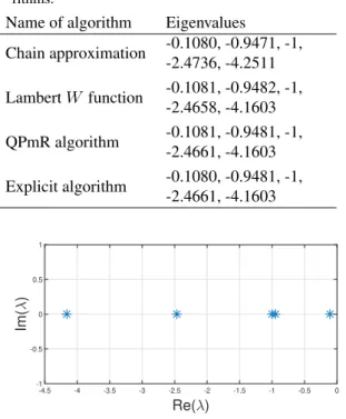
Table 2: The eigenvalues returned by the studied algo- rithms.
Name of algorithm Eigenvalues
Chain approximation -0.1080, -0.9471, -1, -2.4736, -4.2511 LambertW function -0.1081, -0.9482, -1,
-2.4658, -4.1603 QPmR algorithm -0.1081, -0.9481, -1,
-2.4661, -4.1603 Explicit algorithm -0.1080, -0.9481, -1,
-2.4661, -4.1603
-4.5 -4 -3.5 -3 -2.5 -2 -1.5 -1 -0.5 0
Re( )
-1 -0.5 0 0.5 1
Im()
Figure 2:Dominant poles of the DMAS consisting of five agents.
0 20 40 60 80 100 120
Number of iterations (1)
-60 -50 -40 -30 -20 -10 0 10 20 30
tr( n)
tr( n)
|tr(| n)-tr( n-1)|=1e-6
Figure 3: The explicit matrix approximation returns a valid system after12iterations for25agents.
0 to100m, the error of the approximating system is8 cm in the transient domain and5mm under steady-state conditions, as shown inFig. 5.
7. Conclusions
An iterative algorithm was proposed and tested based on which a degree-preserving approximation model can be created for a class of MAS in a platoon formation consist- ing of agents that exhibit first-order dynamics in the pres- ence of a small communication delay. The algorithm uses methods of numerical computation. The obtained MAS is of the same degree and steady state as the delayed MAS, moreover, it correctly approximates the transient behav- ior. The algorithm was compared with existing methods for approximating eigenvalues and systems. Simulations show that the presented algorithm is suitable for the anal- ysis of complex MAS.
0 50 100 150 200 250 300 350 400 450 500
Time (s)
0 10 20 30 40 50 60 70 80 90
Distance (m)
Figure 4:The trajectories of the platoon of the delayed MAS compared to the platoon of the approximated MAS created by the explicit matrix approximation.
0 10 20 30 40 50 60 70 80 90 100
Time (s)
-0.08 -0.06 -0.04 -0.02 0 0.02 0.04 0.06 0.08
Distance (m)
Figure 5:The trajectory of the approximation error.
Acknowledgement
The authors would like to express their gratitude to Dr.
Mihály Pituk (University of Pannonia, Hungary) for his useful comments.
REFERENCES
[1] Kubera, Y.; Mathieu, P.; Picault, S.: Everything can be Agent!, in Proceedings of the ninth Interna- tional Joint Conference on Autonomous Agents and Multi-Agent Systems (AAMAS’2010) (W. van der Hoek, G.A. Kaminka, Y. Lespérance, M. Luck, S. Sen, eds.) (International Foundation for Au- tonomous Agents and Multiagent Systems, Toronto, Ontario, Canada), 1547–1548
[2] Panait, L.; Luke, S.: Cooperative multi-agent learn- ing: The state of the art,Auton. Agents Multi-Agent Syst., 2005 11(3), 387–434, DOI: 10.1007/s10458-005- 2631-2, ISBN: 978-981-10-2491-7
[3] Zabat, M.; Stabile, N.; Farascaroli, S.; Browand, F.:
The aerodynamic performance of platoons: A final report, Institute of Transportation Studies, Research Reports, Working Papers, Proceedings, Institute of Transportation Studies, UC Berkeley, 1995
[4] Cheng-Lin, L.; Fei, L.: Consensus Problem of Delayed Linear Multi-agent Systems, Springer- Briefs in Electrical and Computer Engineering (Springer Singapore), 2017,DOI: 10.1007/978-981-10- 2492-4,ISBN:978-981-10-2491-7
[5] Wim, M.; Silviu-Iulian, N.: Stability and stabiliza- tion of time-delay systems: An eigenvalue-based approach (SIAM), 2007,DOI: 10.1137/1.9780898718645
[6] Lewis, F.L.; Zhang, H.; Hengster-Movric, K.; Das, A.: Cooperative control of multi-agent systems: Op- timal and adaptive design approaches (Springer), 2014,DOI: 10.1007/978-1-4471-5574-4
[7] Trudeau, R.J.: Introduction to Graph Theory, Dover Books on Mathematics (Dover Publications), 2nd edn., 1994,ISBN: 978-0486678702
[8] Chaiken, S.; Kleitman, D.J.: Matrix tree theorems, J. Comb. Theory A, 1978 24(3), 377 – 381, DOI:
10.1016/0097-3165(78)90067-5
[9] Mesbahi, M.; Egerstedt, M.: Graph theoretic meth- ods in multiagent networks, Princeton Series in Applied Mathematics (Princeton University Press), 2010,DOI: 10.1515/9781400835355
[10] Cepeda-Gomez, R.; Olgac, N.: An exact method for the stability analysis of linear consensus proto- cols with time delay,IEEE T. Autom. Control, 2011 56(7), 1734–1740,DOI: 10.1109/TAC.2011.2152510
[11] Arino, O.; Pituk, M.: More on linear differ- ential systems with small delays, J. Differen- tial Equations, 2001 170(2), 381 – 407, DOI:
10.1006/jdeq.2000.3824
[12] Gy˝ori, I.; Pituk, M.: Asymptotically ordinary de- lay differential equations, Functional Differential Equations, 200512, 187–208
[13] Gy˝ori, I.; Pituk, M.: Asymptotic formulas for a scalar linear delay differential equation,Electron. J.
Qual. Theory Differ. Equ., 20161(72), 1–14,DOI:
10.14232/ejqtde.2016.1.72
[14] Krasznai, B.; Gy˝ori, I.; Pituk, M.: The modi- fied chain method for a class of delay differen-
tial equations arising in neural networks, Math.
Comput. Model., 2010 51(5), 452 – 460, DOI:
10.1016/j.mcm.2009.12.001
[15] Corless, R.M.; Gonnet, G.H.; Hare, D.E.G.; Jef- frey, D.J.; Knuth, D.E.: On the Lambert W func- tion,Adv. Comput. Math., 19965(1), 329–359,DOI:
10.1007/BF02124750
[16] Vyhlídal, T.; Lafay, J.F.; Sipahi, R.: Delay sys- tems: From theory to numerics and applications, Advances in Delays and Dynamics (Springer In- ternational Publishing), 2013,DOI: 10.1007/978-3-319- 01695-5
[17] Yi, S.; Duan, S.; Nelson, P.W.; Ulsoy, A.G.: The Lambert W Function Approach to Time Delay Systems and the LambertW_DDE Toolbox, IFAC Proceedings Volumes, 201245(14), 114–119, DOI:
10.3182/20120622-3-US-4021.00008
[18] Vyhlídal, T.; Zítek, P.: Quasipolynomial mapping based rootfinder for analysis of Time delay systems, in Proc. of IFAC Workshop on Time-Delay Sys- tems, TDS 2003,DOI: 10.1016/S1474-6670(17)33330-X
[19] Vyhlídal, T.; Zítek, P.: QPmR – Quasipolynomial rootfinder: Algorithm update and examples, Ad- vances in Delays and Dynamics, vol. 1 (Springer International Publishing, Cham), 2013 299–312,
DOI: 10.1007/978-3-319-01695-5_22, http://www.cak.fs.
cvut.cz/algorithms/qpmr
[20] Latif, A.: Banach contraction principle and its gen- eralizations, Topics in Fixed Point Theory (Springer International Publishing, Cham), 2014 33–64, DOI:
10.1007/978-3-319-01586-6_2