Many-Core Processor

(1)

(2)

Many-Core Processor

Architectures for Topographic Computations

Beyond Parallelism

Ákos Zarándy

Doctoral Dissertation

for the Doctor of the Hungarian Academy of Sciences degree

Budapest

2009

(3)

1 Introduction

The first 8 bit microprocessor, the Intel 8080 applied about 6000 transistors. It ran on 2MHz, and provided 0.5 MOps computational power on 8 bit integers. Following the pace dictated by Moore’s law, the latest microprocessors uses three billion transistors on a single chip nowadays. Their clock frequency goes up to 4 GHz, and they provide 50GFlops on 32 bit floating point numbers. Assuming that 1 Flop @ 32 bit is roughly equivalent with 10 Ops @ 8 bit, we get that a high-end processor nowadays with the given parameters is 1,000,000 (one million) times more powerful than the i8080. This is an amazing technical success indeed!

However, it is worth to calculate the efficiency of the technological usage.

If we look at the transistor counts, we can see that roughly 500,000 pieces of 8 bit microprocessors can be implemented on a single chip nowadays. Moreover, the technology enables to drive them on at least 2000 times higher clock frequency. This means that the technological development offered 1,000,000,000 (one billion) times speed up, and as we have seen, 1,000,000 (one million) times was utilized out of it “only”. The missing 1000 time speedup is very huge, because that is the result of about 15 years of CPU development. How can at least a part of this missing 1000 times performance increase be utilized?

Processor architecture designers are focusing their attention to many core architectures, because neither the further widening of the word length of the super-scalar processors nor the further increase of the clock frequency work due to low efficiency of the formal and very high power consumption penalties of the latter. This initialized a transition in the processor industry towards the multi-core designs. A new Moore’s law estimates that the number of the cores in a single chip doubles in each year [56]. Intel and AMD came out with the duals [60][61] and later the quads for desktops, while IBM and SUN built 9 core processors [58][62] for servers. Other designs reached close to 100 processor cores [63][66]. Nvidia introduced the CUDA processor array family, which goes up to 240 cores [65].

Though this is a very impressive roadmap, we have to know, that there are major problems with the many-core architectures, because the gigantic mass of the nowadays used software, what we would like to use in the future also, cannot be efficiently executed on them.

Moreover, there is no general solution how to modify an algorithm to make it efficiently executed on a many-core device. On the other hand, the optimal many-core processor architecture selection for a given problem in general is also unknown. And top of all that, none has an idea what we can do with ten thousand or even hundred thousand processor cores on a single die, though the readily available CMOS technology makes the implementation of such a mega-processor array absolutely feasible. The answers to these architectural and algorithmic questions are one of the most intensively researched areas of the field, because they will shape the short and midterm development paces of the computer technology.

(7)

In my Dissertation I am addressing one segment of these problems, namely the topographic many core processor architectures, and their application in 2D data array (image) processing. The special feature of these topographic processor arrays is that the processor cores are arranged to the vertexes of a regular grid. This regularity introduces novel phenomena to these processor arrays, namely the appearing physical address of the individual processors and the increasing precedence of the locality (the local interconnectivity). This means that the communication between the neighboring cores becomes much cheaper than the communication among farther cores. This leads to the efficient implementation of the wave- type operators (see later) on these topographic architectures, because the processor boundaries do not raise barriers for the propagating wave-fronts.

One of these architectures is the Cellular Neural/nonlinear Network (CNN). CNN is based on a large number of locally interconnected, identical, programmable, mixed-signal processors cells, arranged to a rectangular grid. The novelty of these devices is, that the cells are dynamical elements, and the aggregate temporal cell dynamics over the array generates spatial-temporal wave phenomena (propagating waves). The array dynamics of these topographic processors introduces operators, which are beyond the Boolean logic [31]. These operators are spatial-temporal dynamic phenomena and their operands are entire images rather than a few scalars. Typical operators from this group are the various feedback convolutions, the diffusion, the global average applied to a whole image, the global OR applied to an entire binary field [42], a single transient centroid, grassfire, or skeleton [48] operation. When the CNN dynamics is embedded in a stored programmable machine (CNN Universal Machine [27]) we can start thinking in spatial-temporal algorithms.

Other special feature of the CNN processor chip is that the data is topographically represented on the processors on a one to one manner. This one-to-one correspondence between pixels and processors makes possible to add sensors to each pixel, which converts the device to a sensor-processor array. The compactness of the mixed-signal processor cores enables to implement relatively large sensor-processor arrays. The two largest are the 128×128 sized ACE16k sensor-processor array [42] containing over 16,000 processor cells (cores), and the 176×144 sized Q-Eye [67].

Though CNN-UM (or “CNN computer”) [27] is a fully programmable Turing machine equivalent device [28], its programming is far from triviality. Programmers have to create templates, which describe the interconnection weights of a dynamically coupled, 2D dynamic processor array in such a way that the trajectories of the resulting coupled differential state equation system lead to the desired output of the particular image processing function. Due to its dynamic coupling, CNN can implement spatial-temporal wave phenomena, including propagating binary waves sweeping through the entire array. In my first thesis, I am introducing a template design method for non-propagating and propagating type binary input-

(8)

In the last few years numerous locally interconnected massively parallel low-power topographic sensor-processor arrays have been designed both in the academic [42][44][49]

and in the commercial [67][68] arena. The common features of them is that all of them is designed to process medium resolution images on very high speed, but they cannot handle high (VGA or megapixel) resolution image flows on video speed. This is due to the lack of enough on-chip memory required by the original 2D processor architecture, rather than the lack of computational power. In my second thesis group, I will introduce the virtual topographic processor arrays, which enable to trade the resolution to speed.

To be able to efficiently design and use multi/many core architectures, we have to answer the major questions, namely which processor arrangement to use in a particular application, and how to implement the algorithm on them. In my third thesis group, I am classifying the wave type operators according to their implementation methods on the different architectures.

Then, I am introducing an architecture selection method.

Thesis I Direct CNN template design

Cellular Neural/nonlinear Networks (CNNs) implement coupled, nonlinear, differential equation systems, which are continuous in time and value, and discrete in space. The template of the CNN lists the free parameters of the network, which is practically the program of this complex array processor. Based on the template value configuration, the region of dependency can be either within the interconnection radius; or within a well defined bounded region, which is larger than the interconnection radius; or it can be the whole CNN lattice without any limitations. In the latter case, the transients of the coupled differential equation system may exhibit spatial-temporal wave propagation phenomena.

Finding appropriate template to solve a certain 2D function is an inverse problem, because it is easy to test, what function belongs to a template, but it is not trivial the other way around. There are various methods for finding these templates. The first is the heuristic, which may or may not lead to some solutions, which are usually not optimal. The second is the template learning with different methods (back propagation [34], genetic algorithms [33], gradient based method [34], etc). These methods often require long iteration sequences, and lead to sub-optimal solutions only, if they find solution at all. Since the template space is extremely huge, due to the 19 free variables for the simplest CNN, the brute-force method is not an option. The last method is the direct template design, which leads to optimal solution by using a few closed forms. I have derived these forms for binary-input Æ binary-output templates.

I. I have developed a method for directly designing optimal binary-input Æ binary- output CNN templates for both non-propagating and propagating cases [1]. The method reduced the inverse problem of the CNN template design to the solving of

(9)

a set of inequalities. The advantage of the method is that it leads to the optimal (most robust) template.

I.1. I have proved that in case of binary-input Æ binary-output propagating type templates, the pixel transition is strictly monotonic if the off-center A template elements are positive, and a00>1, and mono-directional cell transitions are enabled only.

I have introduced global rules, which were derived from the properties of the particular wave. These global rules were then transformed to local rules, and later to activation patterns.

These activation patterns were template sized binary or symbolic patterns, which defined those local binary pixel arrangements were the output was supposed to change. I showed that even propagating case wave phenomena can be described using such activation patterns. I have classified the binary-input Æ binary-output templates, and showed how to generate template forms, and then systems of inequalities from the activation patterns.

Thesis II Virtual topographic processor arrays for space to time conversion

Topographic array processors, such as classic CNN computer chips, can efficiently utilize thousands of parallel processors, and can even process medium sized images above 10,000 FPS easily using less than 1 Watt. Unfortunately, this extremely high image processing performance and efficiency cannot be traded to higher resolution–lower speed operation mode due to inherent architectural constraints of the topographic arrangement.

The problem is rooted in the fact that the data is distributed in the 2D topographic array among the processor cells and each processor cell handles one pixel (fine-grain), or a small image segment (coarse-grain). This requires keeping the entire image in internal local memory, otherwise each of the processor cells needs parallel access to external memories during the operation, which is impossible considering couple of hundreds or thousands processors on a single chip.

I bridged the problem by showing different virtual high resolution topographic arrays.

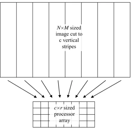
The physical processor engine, behind the virtual processor array is a medium resolution topographic processor array. This physical processor array is allocated to different parts of the virtual processor array from time to time. The allocation can be either periodical or non- periodical. In the latter case, it is image content dependent. The topology of the physical processor array and its communication methods depend on the approach and the parameters such as resolution, pixel clock, signal domain, neighborhood size, and functionality. Beyond the general idea, I have explored four particular arrangements.

(10)

II. I have described the virtual topographic processor array concept. Two approaches have been introduced for the time-to-space conversion of the topographic computer arrays. The first is a sequential approach for early image processing, while the second is the foveal approach for post processing.

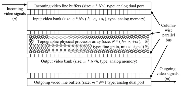
II.1.1 I have introduced a virtual processor array architecture for analog video image processing. The special feature of the architecture is that it does not digitize the analog video signals. Behind the 2D full video frame size virtual processor array, there is an elongated mixed-signal physical processor array [4].

II.1.2 I have proposed a virtual processor array architecture for calculating high speed CNN operation in the digital domain. The physical processor array is the CASTLE [2] architecture, which can achieve calculations in 3 different bit depths. The virtual processor array can handle various image sizes, and can implement space variant template operations.

II.2.1 I have showed how the foveal concept can be implemented by using ultra-high speed, low resolution CNN chip as physical device. This virtual processor approach bridged the gap between the 10,000 FPS low resolution image processing, and the video speed high-resolution image processing. With the help of the ultra-high speed, low resolution CNN chip, 1000 FPS foveal image processing was performed in high-resolution images.

II.2.2. Monolithic, ultra-low power, ultra-high performance sensor-processor chip is proposed for performing airborne navigation tasks. The novelty of the device is that it combines a medium resolution mixed-signal processor array for early image processing, and a digital foveal processor array for post processing. The single chip implementation was made possible by using the new 3D silicon integration technology.

Thesis III Low-power processor array design strategy for solving 2D topographic problems

Low-power topographic processor arrays are widely used in the image processing field nowadays. Their characterization and comparison is an important task, when someone wants to select one of them to apply in a particular application. However, it is quite complicated since they have drastically different architectures, operation modes, and parameters. To be able to make this comparison, I have analyzed the most important low-power topographic and non-topographic multi- and many-core architectures, and then, I have classified the basic image processing operators, including the wave computing ones, according to their

(11)

implementation methods on these architectures. Based on these results, I gave an optimal multi- or many-core architecture selection methodology.

III.1. I have classified the most important 2D operators, including the wave computing ones, based on their implementation methods on different topographic and non- topographic multi- and many-core image processing architectures. The most distinguishing features were the activity pattern distribution of the pixels (front active versus area active), the content dependency of the waves, and the spatial- temporal calculation method of the operators.

III.2. I have determined the computational efficiency of these 2D operators, on various topographic and non-topographic multi- and many-core image processing architectures. Moreover, I have calculated the computational demand, the execution time, and the latency values of the operators executed on the different topographic architectures.

III.3. I have derived an optimal multi- or many-core image processing architecture selection methodology. The method is based on the characteristic features of the given algorithms, namely the frame-rate, latency, resolution, instruction types, and the structure of its flow-graph.

(12)

(13)

(14)

2 Direct CNN template design

A Cellular Neural Network (CNN) [26] is a locally interconnected analog processor array arranged to regular 2D grid. Its two-dimensional inputs and output make it extremely suitable for image processing. Due to its regular (in most cases rectangular) arrangement and its local interactions, programmable CNN (the so-called CNN Universal Machine [27]) can be efficiently implemented on silicon. With the today available deep-submicron technology 128×128 sized analog processor arrays have been implemented on a single chip [42]. The spatial-temporal transient of an analog VLSI CNN array settles down in the microsecond range. This means that an image processing primitive (like edge detection, blurring, sharpening, thresholding, etc.) can be calculated for a 128×128 pixel sized image in a few microseconds on a single low-power chip. This speed enables to implement image processing algorithms and real-time visual decisions over 10,000 FPS in the embedded space, which is unique. But while programming conventional digital computers is relatively easy, here one has to find an appropriate parameter set of a continuous time spatial-temporal nonlinear processor array to force its dynamics to calculate an image processing primitive. Since CNN has space invariant local interconnection structure it has a few dozens free parameters only, depending on the sphere of influence. This parameter set, called template, exclusively determines its array dynamic behavior.

There are three major template design methods: (i) intuitive, (ii) template learning, and (iii) direct template design. The first requires intuitive thinking of the designer. In some simple cases it leads to quick results, but typically not to the optimal one. On the other hand, it does not guarantee to find the desired template at all. Moreover, designers need to have lots of experiments in both the image processing and the array dynamics.

The second design method, the template learning, is an extensively studied, popular field of the CNN research. Almost all classic neural network training methods have been adapted to the CNN structure. But there are three serious problems with these techniques and results.

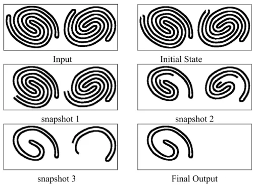
First of all, the learning is based on input and desired output pairs and during the learning procedure better and better results are supposed to be generated with better and better templates. But in many cases (especially binary propagating type templates like CCD shown in Figure 16 [23]) a template either works or does not work, and there are no gradual better and better result series. This changes the strategy of a learning method to a brute-force one.

The second problem is that in some cases the template for the given problem does not exist.

The learning methods cannot even realize it and run forever. If the template exists, it might take a long time to find it, if it can at all. The third problem is that several proposed learning methods were tested and proved to be efficient to those template classes, which can be directly derived from the exact function descriptions. In these cases it is unnecessary to use learning methods. However, there are some cases when the template learning is a very

(15)

important design method. In these cases, no explicit desired output exists, hence direct template design is impossible. Texture separation is a good example for this case [51].

The third method, what I have introduced, is the direct template design. It can be applied when the desired function is exactly specified. The design methods depend on the particular template class. While the previous two methods produce a single or a few operational templates, here we get all of them. This provides the opportunity to choose the most robust one among them. Moreover, this method needs only a small fraction of the computational power with respect to the template learning needs.

All template design methods, presented in this paper, can be used in both the Chua-Yang model [24] and the Full Signal Range (FSR) model [36]. In case of the FSR model the center element of the derived template should be decreased by 1.

In this chapter, first a brief description of the CNN will be given. This will be followed by the uncoupled binary-input Æ binary-output CNN template design. Finally the coupled binary-input Æ binary-output CNN template design closes the chapter.

2.1 The Cellular Nonlinear/Neural Network model A CNN is defined by the following principles:

• A set of spatially coupled dynamical cells arranged to a 2D grid, where information can be loaded into each cell via two independent variables called input (u) and the initial state (x(0)). In this way, the CNN is continuous in time and value, and discrete in space.

• The behavior of the network is defined by the coupling law which describes the relation (weight coefficient) between one or more relevant variables of each cell to all local neighboring cells located within a prescribed sphere of influence Sr (i,j) of radius r centered at cell (i,j). This set of coupling laws, called template, is space invariant for the whole grid.

Figure 1a shows a CNN composed of cells that are connected to their nearest neighbors.

Due to its symmetry, regular structure and simplicity this type of arrangement (rectangular grid) is primarily considered in all implementations.

(16)

j^th column

i^th row

x_ij - state/ y_ij - output

z - bias

uij - input

(a) (b) Figure 1. A 2-dimensional CNN defined on a square grid (a). The i,j-th cell of the array

is cyan, whereas cells that fall within the sphere of influence of neighborhood radius r = 1 (the nearest neighbors) are pink. The two layers of the CNN and their internal interconnections are shown in (b). The red arrows represents the feed forward weights, while the blue ones the feed-back. The green arrow shows the space invariant bias.

Figure 1b shows the two layers of the CNN. The lower layer is the input, which is typically constant in time. The upper one represents the dynamically changing state and output layers.

They are indicated as a single layer because they are strongly bonded (see equation 2.2). The external single source is a constant bias. The electrical circuit of the cells is shown in Figure 2. The cell dynamics is described by the following nonlinear ordinary differential equations:

State equation:

2.1

( ) ( )

( )

, , , ,

; ( ) ;

r r

k l S i j l k l S i j

x t 1x t z A y t B u

ij ^{= −}τ ij ⁺ ij ⁺ _∈

∑

ij k ^⋅ kl ⁺ _∈

∑

ij kl^⋅ kl

& t

−

(2.1) Output equation:

2.2

( ) ( )

( ) ( ) ( )

1 if 1

( ) if 1 1

1 if 1

x t ij

y t f x t x t x t

ij ij ij ij

x t ij

⎧ >

⎪⎪

⎛ ⎞

= ⎜⎝ ⎟⎠ ⎪=⎨ − ≤

⎪− <

⎩

≤ -1 1

-1 1

x_ij yij

(2.2)

where

• xij, yij, uij are the state, the output, and the input variables of the specified CNN cell, respectively. The state and output vary in time, the input is static (time independent), ij refers to a grid point associated with a cell on the 2D grid, and kl ∈ Sr is a grid point in the neighborhood within the radius r of the cell (i,j).

• zij is the threshold (also referred to as bias) which is constant in space and time.

(17)

• Term Aij,kl represents the feedback, Bij,kl the control weight coefficients. These are scalar matrices, which are constant in space and time during a transient.

• τ is the cell time constant, for simplicity we consider τ =1/RC= 1.

• Function f (.) is the output nonlinearity, in our case a unity gain sigmoid. It has three regions. The middle region is called linear region, while the two other regions are called saturation regions. The CNN terminology calls an output value grayscale, when it is in the linear region, and binary value, when it is in one of the saturation regions.

• t is the continuous time variable.

±

zij

R

u_ij yij

R C

x_ij

A_ij,kly_ij Bij,kl uij

input state output

Figure 2. The equivalent circuitry corresponding to the CNN state and output equations as it is defined in (2.1). The control and feedback terms are represented by voltage controlled current sources (Bij,kl and Aij,kl).

The state equation (2.1) and the output equation (2.2) define a coupled nonlinear differential equation set, which is a rather complex framework for computation. The first part of the state equation is called cell dynamics, whereas the additive terms following it represents the synaptic interactions.

The time constant of a CNN cell is determined by the linear capacitor (C) and the linear resistor (R) and it can be expressed as τ = RC. A CNN cloning template, which can be considered as the instruction on the CNN array, is given by two weight coefficient matrices and a bias term (for example see equation 2.3) implemented by the voltage controlled current sources.

2.3 , , ; (

1 , 1 0 , 1 1 , 1

1 , 0 0 , 0 1 , 0

1 , 1 0 , 1 1 , 1

1 , 0 0 , 0 1 , 0

1 , 1 0 , 1 1 , 1

i z b

b b

b b b

a a a

=

⎥⎥

⎥

⎦

⎤

⎢⎢

⎢

⎣

⎡

=

⎥⎥

⎥

⎦

⎤

⎢⎢

⎢

⎣

⎡

=

−

B

A 2.3)

In order to specify fully the dynamics of the array, the boundary conditions have to be defined. Cells along the edges of the array may see the value of cells on the opposite side of the array (toroidal boundary), a fixed value (Dirichlet-boundary) or the value of mirrored cells (zero-flux boundary).

(18)

2.2 Uncoupled CNN templates

Uncoupled templates have zero off-center A template elements only. The general form of the uncoupled templates is the following:

2.4. A= B (

⎡

⎣

⎢⎢

⎢

⎤

⎦

⎥⎥

⎥

=

⎡

⎣

⎢⎢

⎢

⎤

⎦

⎥⎥

⎥

=

− − − −

−

0 0 0

0 0

0 0 0

00

1 1 10 11

0 1 00 01

1 1 10 11

a

b b b

z i

, , 2.4)

Since their dynamic parts are uncoupled, they work as an array of independent first-order elements (cells). Hence, it is satisfactory to analyze the dynamic behavior of a single cell only. A single cell receives 9 static inputs from the input layer (u_kl). It has an initial condition x(0), which can be considered as a tenth input. An uncoupled CNN cell maps these 10 inputs to a single output, with other words it implements a 10 input one output function. The state equation of a single cell is as follows:

2.5

&( ) ( ) ( )

x t x t a y t s z

= − + +

; ( )

, ( ) ( , )

s u

y f x

ij kl C kl N i j

kl

r

= +

=

∑

∈ ^B ⁰⁰ ^-1 ¹

-1 1

x f (x)

&

(2.5)

Where: s is a constant during the transient evaluation, which depends on the template and the input of the CNN; f is the output characteristics, a sigmoid function in our case. The flow- graph which describes the first order, differential system of a single cell can be seen in Figure 3.

x x

Σ ∫

^y

a₀₀ -1 s

Figure 3. The flow-graph of the first order system of a single cell.

Before going on with the dynamic analysis of a single cell, let us describe the errors and deviations coming from the analog implementation of the CNN. In case of the analog implementation, the template parameters of the CNN are slightly varying. This can be considered as each cell has an individual template. Although all the template values are close to the nominal ones the difference of any measurable template value and the corresponding nominal one changes from value to value and cell to cell, but they are constant in time. Their distribution and deviation depends on the particular chip piece.

(19)

The dynamics of a cell depends on the a₀₀ parameter. First let us see the dynamic response of the cell quantitatively, via solving the ODE in the linear region (x=y).

2.6. x&+ −(1 a x) =s (2.6)

2.7. 1: ( ) ⁽¹ ⁾

1

if a x t ce a t

a

≠ = + − −

− s

+

(2.7)

2.8. if a=1: x t( )=

∫

sdt+ =c st c ^(2.8)

After the quantitative analysis, let us do a qualitative analysis of the practically important cases. We call the following statements rules, and we will recall them later on. These are as follows:

Rule 1. a₀₀=0. In this case the final state of the cell is equal to the input ( x_∞=s ), hence the final output is y_∞=f(s).

Notes: 1. The final output is independent of the initial state x(0).

2. The transient settles with an exponential decay in the linear region.

3. The output will be binary if and only if |s|>1.

Rule 2. a₀₀=1. In this case the CNN behaves as an integrator, while x is in the linear region (|x|<1). Ideally, if s≠0, then the final output depends on the sign of s, i.e.:

y_∞=sign(s). If s=0, then the final output depends on the initial state, i.e.: y_∞=x(0).

However, due to the given mismatch and other non-idealities of the analog VLSI implementation of the circuit, we have to use |s|>ε>0, to get y_∞=sign(s). (ε is larger than the largest template mismatch value)

Notes: 1. If |s|>ε>0, then the final output is independent of the initial state x(0), and it is binary.

2. If |s|>ε>0, then the output saturates in less than 2s time (starting from the linear region). In this case the transient decay is linear in the linear region.

3. In practice, we have to avoid the use of the s=0 case, because in case of an analog realization the precise equality is not a valid possibility, hence the final output will depend on unpredictable parameter deviations.

Rule 3. a₀₀>1, usually 2 or even higher. The final output is always binary, due to the positive feedback loop. The final output depends on the initial state and the

(20)

contribution of the input (s). There are three practically important cases. The last discussed case is the general case.

(a) x(0)=0 hence y(0)=0. The final output depends on the sign of s, i.e.:

y_∞=sign(s). In this case the initial feedback is zero. The integrator starts increasing or decreasing according to the sign of s, and due to the positive feedback, it will go to one of the saturation zones.

(b) x(0)=+1 hence y(0)=+1. The final output remains +1, if a₀₀+s-1>0. The final output changes to -1, if a₀₀+s-1<0.

(c) x(0)=-1 hence y(0)=-1. The final output remains -1, if -a₀₀+s+1<0. The final output changes to -1, if -a₀₀+s+1>0.

(d) x(0)=x₀, where |x₀|<1, hence y(0)= x₀. The final output depends on the sign of , precisely: y_∞=sign( )=sign((a₀₀-1)x₀+s).

(This case is the generalization of the previous ones.)

&( )

x 0 x&(0)

Note: The a₀₀+s=1 situation and the -a₀₀+s=-1 situation should be avoided in practical cases, because in case of an analog implementation the precise equality is not a valid possibility, hence the final output will depend on unpredictable parameter deviations.

These rules can be trivially derived from the state equation (2.5) and the flow-graph (Figure 3.) of a single CNN cell. After analyzing the dynamic of a single cell, here we go through the elementary uncoupled CNN template classes. From now the inputs and the outputs of the CNN will be presented in image forms. We follow the original convention of [24], where +1 stands for black, and -1 stands for white, and the intermediate values are represented by different gray shades.

2.2.1 Binary-input Æ binary-output uncoupled CNN templates

The uncoupled binary CNN templates form a very important class of the CNN templates, because they cover many different frequently used image processing tools, including the binary mathematical morphology. The family of operations can be separated into two main groups. The first is the single input (e.g. constant zero initial state, image on input layer only), while the second is the two input (images on both the initial state and the input layers).

During the discussions of the template design methods, first we introduce the design for some special template classes, and then the general solution will be discussed. These template classes are important, because they are simpler than the general solution, hence the template design methods are simpler too, and moreover they cover most of the practical templates. We will also give the list of the templates from the Template Library [23] belonging to the each design classes.

(21)

Class I. Single input image, equal pixel roles

This class of templates extracts 3×3 unweighted pattern combinations. (Unweighted means that the individual elements play the same role). When describing the problem a binary 3×3 pattern and a limit (integer number) are given. The binary pattern contains black pixels, white pixels and “don’t care” pixels (See example in Figure 4.). The given limit controls that at least how many positions of the pattern should match to set a pixel.

The black-and-white input image is placed to the input of the network. The initial state is set to zero. At the end of the operation, the output is black in those pixel positions, where the number of matches was equivalent or exceeded the given limit.

Design example A:

Given the 3×3 binary pattern shown in Figure 4a. Suppose that the threshold value is 5.

9 9 9 9

X

9

(a) (b) (c)

Figure 4. Example for binary pattern matching. (a) shows the binary pattern. Squares with ‘-’ means, “don’t care”. (b) shows the test pattern. (c) shows the matching and the non-matching pixel locations. The matching positions are denoted with ‘9’ and the non-matching one with ‘X’. Since, there are 5 matching positions, the output of the cell will be black (+1).

The design steps of the uncoupled CNN templates are shown by the flowchart in Figure 5. The first step is the most important, because the key of the successful template design is the correct template form determination. As we saw in (2.4), generally there are 11 free parameters of the uncoupled CNN templates. When we determine the template form, we drastically reduce the number of the free parameters. Some of the parameters will be set to zero, and some groups of it will be handled together. With this method the number of the free parameters is usually reduced to 3 or 4. This means that in usual cases the template space is reduced to a 3 or 4 dimensional one. See (2.9) for the template form of the design example 1!

template form determination

generate a relation system

solve the relation system

choose the most robust template Figure 5. The flowchart of the design method of the binary input-binary output

templates.

(22)

The second step of the template design is the generation of a system of inequalities. It can be derived automatically from the task and the Rules. Each inequality guarantees the output to a certain input configuration. Since the input-output pairs are known, the generation of the system of inequalities is simple. Each relation defines a hyper plane, which cuts reduced template space into two halves. The inequality is satisfied in one half only. Since all the inequalities should be satisfied, the intersection of the half spaces contains the correct templates. If it is an empty set, the function cannot be solved with a single template (linearly not separable function [29]) in the determined template form. A graphical visualization example can be seen in Figure 6a, and will be explained in the next example.

Template form determination:

After the general idea of the design method was explained (Figure 5) let us show it in practice in Example I. First of all, the template form should be determined. The template form can be directly derived from the binary pattern (Figure 4a). a₀₀ will be larger than 1 (say 2) which guarantee that the final output will be binary (Rule 3.). The initial condition will be set to zero, hence the final output will be sign(s) (Rule 3a.). In template B, the don’t care positions are equal to zero. All the black positions play the same role, hence, they can be denoted with the same free parameter, say b. The role of the white positions are exactly the opposite of the role of the black positions, hence they will denoted by -b. The template is sought in the following form:

2.9. A= B (

⎡

⎣

⎢⎢

⎢

⎤

⎦

⎥⎥

⎥

=

− −

⎡

⎣

⎢⎢

⎢

⎤

⎦

⎥⎥

⎥

= 0 0 0

0 0

0 0 0

a b b b

b b b

z i

, , 2.9)

System of inequalities:

After determining the form of the template the generation of the system of inequalities is straightforward. One has to go through all the possible combinations of the input patterns, and apply the particular Rule, in our case Rule 3a. This means that the initial state is zero, and the sign(s) determine the final output. Numerically we can distinguish 7 different cases depending on the number of the matching pixels.

# of matching pixels desired output relations

6 black (+1) 6b+i>0

5 black (+1) 4b+i>0

4 white (-1) 2b+i<0

2.10. 3 white (-1) i<0 (2.10)

2 white (-1) -2b+i<0

1 white (-1) -4b+i<0

(23)

Solution of the system of inequalities, and selection of the most robust template:

Fortunately in this case there are only two free parameters of the system, hence we can solve the problem graphically. The graphical solution can be seen in Figure 6a. By solving the system of inequalities we get an infinitely large subspace, from which we have to pick a single point to be the nominal template. By testing different templates from the found region in simulator, we can see that the convergence of some templates will be faster, others will be slower, but all templates in the specified template sub-space will work fine. But if we want to apply our templates on a CNN chip we have to consider the parameter deviations coming from the analog implementation. As we saw at the beginning of this section, the parameter deviation can be considered as each cell would have an individual template, which is close to the nominal template. To select the most robust template, we have to consider the followings:

• It is a rule of thumb that the more we scale up the template values, the faster the transient will be.

• Due to local silicon process variants, we suppose that the template values in a CMOS chip will be within a circle around the nominal template. To guarantee the robustness of the template this circle should be inside the specified subspace with its total volume. On the other hand, it can be seen that the subspace opens (becomes wider) if the values are scaled up.

• The analog implementation of the CNN always limits the maximal absolute value of the template elements. Let say that in our case the absolute value of a template element should not exceed 3 and the absolute value of the bias (current) should not exceed 6. It is the case in [42]. This limits the infinite subspace to a finite subspace. These boundaries are denoted with dashed lines in Figure 6b.

Hence, we have to choose the largest possible b and i value from the middle of the subspace. These values (b=2.2, i=-6) determine the selected template. We call the selected template as the nominal template. The real templates will be around it in the circle. The chosen best template is the following:

2.11. A= B (

⎡

⎣

⎢⎢

⎢

⎤

⎦

⎥⎥

⎥

=

− −

⎡

⎣

⎢⎢

⎢

⎤

⎦

⎥⎥

⎥

= − 0 0 0

0 2 0 0 0 0

0 0 0

2 2 2 2 2 2 2 2 2 2 2 2

6

, . . .

. . .

, z 2.11)

Notes:

1. The specialty of this template class is that template B contains one free parameter only, hence it is constructed from zero, a certain real number and its opposite.

(24)

2. From the robustness point of view, it is more difficult to implement the template, if the threshold number is larger (6 instead of 5 in our case), because it makes the result template subspace narrower. In Figure 6a, this subspace is the narrow one below the shaded part. If the resulting template subspace is narrower, it might be difficult to keep the circle of tolerance with its total area inside.

b

-3 i

1

-2

3 1

2 3

-1

-3 2b+i<0

4b+i>0 6b+i>0 -6b+i<0 -4b+i<0 -2b+i<0 i<0

b

-6 2 i

2 4 6

-4 -2 -2 nominal

template

(a) (b) Figure 6. (a): Graphical solution of the system of inequalities (2.10). All of the

inequalities are represented with a straight line, which divides the plane to two halves. The arrows on each line indicate that half, which satisfies the particular inequality. The union of the half plans is the solution subspace (shaded). (b): Selection of the nominal template. The dashed lines show the technical limitations of the ACE16k chip. The ‘×’ shows the chosen best nominal template, and the circle around it contains the real templates.

Templates from the Template Library [23], which belong to this class:

EROSION, DILATION, DELVERT1, DIAG1LIU, FIGDEL, LSE, PEELHOR, RIGHTCON. (Some of these templates are described in the Appendix.)

Class II. Design method of the one input image differential pixel roles

In the previous case, all the pixels played the same role, and the decision was made on their matching statistics. Here, we have two groups of active pixels. The first pixel group contains the priority pixels, which must match anyway, while the second group contains the non-priority pixels, from which only a given number is required to match. In this template class, a binary pattern (with indicated priority, non-priority, and don’t care positions), a threshold (limit) number, and a rule whether to change white pixels to black or black pixels to white are given. When the number of the matching positions is calculated the non-priority positions should be concerned only.

(25)

Design example B:

Given the 3×3 binary pattern shown in Figure 7a. The task is to set those locations to white, where the priority pixel and all the five non-priority pixels matches, and keep the original value otherwise. Figure 7b and c show an example. (The example template is the first one from the skeletonization template series [23].)

np np

np np p

np ^X 9

9 9 9

(a) (b) (c)

Figure 7. (a) is the given binary pattern with the indicated priority (p), non-priority (np) and don’t care (-) positions. (b) is the test pattern. (c) shows the matching and the non-matching pixel locations. Since, there are 4 matching positions in the non-priority region the output of the cell will not change. Note that when the matching positions are calculated the priority pixel position is not concerned.

Template form determination:

The template form can be directly derived from the binary pattern (Figure 7a). a₀₀ will be larger than 1 which guarantee that the final output will be binary (Rule 3.). The initial state will be zero, hence the final output will be determined by Rule 3a (the sign of s). In template B, the don’t care positions are equal to zero. The specialty of this class is that the priority positions of template B play different role than the non-priority positions. The reason is that all of the priority ones are supposed to match. Hence, the priority pixel positions of template B always get a new free parameter, (say b).

The black non-priority positions play equivalent roles, hence they can be characterized by the same free parameter, name it c. The role of the white non-priority positions play exactly the opposite role than the black positions, hence they will be -c. The template is sought in the following form:

2.12. A= B (

⎣

⎢⎢

⎢ ⎦

⎥⎥

⎥

= −

⎣

⎢⎢

⎢ ⎦

⎥⎥

⎥

=

0 0

0 0 0 0 0

a c b c

c

z i

, ,

⎡0 0 0⎤ ⎡−c −c 0⎤

2.12)

System of inequalities:

Since the initial state of the CNN is zero here and a₀₀>1, we have to consider Rule 3a.

Here the number of the relations will be (Np+1)*(Nnp+1), where Np and Nnp are the number of the priority and non-priority positions respectively. In our example, the inequalities are as follows:

(26)

self input (priority)

# of matching non- priority pixels

desired output relation

black (+1) 5 white (-1) b+5c+i-1<0

black (+1) 4 black (+1) b+3c+i-1>0

black (+1) 3 black (+1) b+c+i-1>0

black (+1) 2 black (+1) b-c+i-1>0

black (+1) 1 black (+1) b-3c+i-1>0

2.13.black (+1) 0 black (+1) b-5c+i-1>0 (2.13)

white (-1) 5 white (-1) -b+5c+i+1<0

white (-1) 4 white (-1) -b+3c+i+1<0

white (-1) 3 white (-1) -b+c+i+1<0

white (-1) 2 white (-1) -b-c+i+1<0

white (-1) 1 white (-1) -b-3c+i+1<0

white (-1) 0 white (-1) -b-5c+i+1<0

After solving the system of inequalities, the resulting template is as follows:

2.14 , 0.5

0 5 . 0 0

5 . 0 5 . 2 5 . 0

0 5 . 0 5 . 0 B , 0 0 0

0 2 0

0 0 0

−

=

⎥⎥

⎥

⎦

⎤

⎢⎢

⎢

⎣

⎡

−

=

⎥⎥

⎥

⎦

⎤

⎢⎢

⎢

⎣

⎡

= z

A (2.14)

CORNER,EDGE,SKELETONIZING,CENTER,FIGEXTR,JUNCTION,CONCAVE Class III. Two input images

The specialty of this class is that both the input and the initial state of the CNN carries two different relevant images, hence an additional input appears, and the total number of the pixels, which affects the final output is 10 (instead of 9 like in the previous two classes). The image downloaded to the initial state of the network can be considered as a mask. This means that we cannot define a neighborhood operation on the initial state. Rather than that, through this image, we can modify the local neighborhood functionality applied to the other image downloaded to the input.

On the other image, downloaded to the input, the same spatial functions can be defined what we saw in the previous two classes. The resulting image of this function and the initial state can be logically combined with the same template.

The general solution of this class is as follows. If we consider Rule 3b and c, we find that

(27)

2.15. w_{0 0}+ s >0 i f x( 0) =+ 1 (2.15)

2.16. - w_{0 0}+ s > 0 i f x(0)=-1 (2.16)

Here we used a00 = 1+w00, because the ‘1’ is used for the compensation of the integrator in the linear region, and the remaining w00 is the real weight coefficient. Similarly, the final output is -1, if:

2.17. w_{0 0}+ s <0 i f x( 0) =+ 1 (2.17)

2.18. - w_{0 0}+ s < 0 i f x(0)=-1 (2.18)

The consequences of the above expressions are:

y∞=-1 if s<- w00

2.19. y∞=1 if s> w00 (2.19)

y∞=x(0) if - w00 < s < w₀₀

This leads to a hysteresis behavior, as it is shown in Figure 8. The output depends on the logic combination of the contributions of the input and the initial state. Three kinds of logic combinations are possible:

• AND, if s< w₀₀

• OR, if s> -w00

• The third one is a non-standard logic. In this case s can extend the range of [- w00, w₀₀] in both directions. The output will be defined by the contribution of the input in that cases when |s| > |w00|, otherwise it will be x(0).

-w

00

-1 1

s y

_final

w

₀₀

x(0) = -1 x(0)=1

Figure 8. Hysteresis phenomenon can be found in the final output of the binary-input Æ binary-output, two-input, uncoupled CNNs when the self feedback is larger than 1.

LOGAND, LOGDIF, LOGOR, LOGORN.

(28)

2.3 Coupled CNN templates

A CNN with coupled template has array dynamics. The change of the output of an individual cell effects its neighbor's output and vice versa. The array dynamics is described by the coupled first order differential equation system [24] shown in (2.20). The output characteristic, called sigmoid function, is also sown in (2.20). The u, l, and p letters denotes the negative saturation, the linear, and the positive saturation regions respectively, while the N and the P indicates the negative and the positive break points.

2.20

& ( ) ( ) ( )

; ( )

, ( ) ( , )

x t x t y t s

s u z

y f x

kl

r

= − + +

= +

=

∈

∑

A

B

^-1 ¹

-1 1

x f (x)

n N

l P p

(2.20)

We separated the contribution of template B and the bias term, because they are constant during the spatial-temporal dynamics. In this section, we suppose that a₀₀>1.

A coupled Cellular Neural Network structure allows propagation phenomenon. The propagation always works in such a way that only some cells are active and the rest are inactive, in the array. The active cells may or may not activate their inactive neighbors, and after a while they became inactive again. The activated neighbors may or may not activate new neighbors, and the wave propagates as long as active cells can find new neighbors to activate.

A cell is considered to be inactive in a certain time instant, if it is in a stable equilibrium point. The state value of an inactive cell must be in the saturation region (n or p), because due to the positive self-feedback (a₀₀>1), the cell cannot be in a stable equilibrium point in the linear region [24]. Rule 4 describes the necessary conditions for a cell to be stable in the saturation region.

Rule 4. As it follows from (2.20) a cell is stable in the positive saturation region (p) if the value of the term is larger than +1, or it is stable in the negative saturation region (n), if this value is smaller than -1.

A_{ij kl}

C kl N i j kl

r

y t s

, ( ) ( , )

( )

∑

∈ ⁺

A cell is considered to be active in a certain time instant, if its output is changing. The state of an active cell is always in the linear region. Rule 5 shows the necessary condition to activate a cell.

(29)

Rule 5. A cell (pixel) leaves a saturation region under the following conditions:

(a) a cell leaves the positive saturation region (moves from p to l by crossing P),

if:

2.21.

< 1; (

A y ( )t s

∑

⁺

A y ( )t s

∑

⁺

≠00 kl ij kl C kl N i j

kl

r

, ( )∈ ( , )

2.21) (b) a cell leaves the negative saturation region

(moves from n to l by crossing N),

if:

2.22.

> -1. (

kl

r

, ( )∈ ( , )

2.22) In most cases, an activated cell migrates from one saturation region to the other, typically on a monotonic way. Certainly, in some propagating waves some pixel arrangements produce situations, in which cells go into the linear region from one saturation region, and after a while, it changes course and go back to the same saturation region, where it was coming from.

However, in these cases, the final output cannot be unambiguously derived from the input in real analog CNN implementations, because the fact, whether a cell changes course or not, may depend on the local noise of the analog cell (See Section 2.3.1.2). Therefore, it is better to use waves, where such situations are excluded.

We can distinguish propagating waves (template configurations), which enable only one directional (mono-directional) cell transition, and those, which enable both. Though the proposed method can generate templates for both kinds of propagating waves, it is better to design templates for one directional cell transitions, because in that case, one can make sure that the cells will monotonically cross the linear region, making the output an unambiguous function of the input. Rule 6 shows the necessary conditions, which allow mono-direction cell transition only. The specialty of Rule 6 is, that it is defines this property by using template values purely.

Rule 6. A cell is stable in the positive saturation region (p) if the derivative of its state cannot be negative in the positive break point (P):

2.23. ( ) ( ) ( ) 0 (

,

, , ,

, ,

00 + + + ≥

=^w ^y ^t

∑

^y ^t

∑

^u ^z

t x

kl ij

kl ij kl ij kl

ij

kl ij kl ij ij

ij A B

& 2.23)

where w00=a00-1, and xij= yij=1

Since the absolute value of y and u cannot be larger than 1, the following inequality guarantees that (2.23) is always true, when yij=1:

(30)

2.24. ⁺ ^≥

∑

^≠ ⁺

∑

kl kl ij kl

kl kl

z ij

w _,

00 ,

00 A B (2.24)

Similarly, a cell stays the negative saturation region (n), if the following inequality is true:

2.25. ₀₀ ⁰⁰ _, _,

kl

ij kl ij kl

kl kl

w z

+ ≤

∑

≠ ^A +

∑

^B ^(2.25)

Note: Rule 6 states that under certain conditions, derived from the template and not the neighborhood pattern only, a cell cannot leave one of the saturation region. Hence, cells, which are in that saturation region, cannot be activated. However, it does not state anything about states, which are in the other saturation region. Those may stay, may leave, according the local neighborhood pattern.

After defining the necessary condition of the mono-direction cell transition, we examine what is required to guarantee the strictly monotonic cell transition.

Theorem 1. Assuming that only mono-directional cell transition is enabled (Rule 6 satisfied), and a00>1, and the off-center A template elements are positive, the pixel transition is strictly monotonic.

Proof: We are using an indirect proof here. We will prove the theorem for negative to positive cell transition. Since it is symmetric, it can be proved for the other direction similarly.

In t0 some of the cells leave the negative saturation region, and the spatial-temporal transient starts. Assume that cell (ij) is the first cell in the array, which changes course, and starts heading back to the negative saturation region. Let us denote the time instant with t1, when cell (ij) left the negative saturation region, and t2, when it changes course.

In t1, we know that

2.26. ( ) ( ) ( ) 0 (

,

, , 00

,

1 , , 1

00

1 =^w ^y ^t +

∑

^≠ ^y ^t +

∑

^u +^z>

t x

kl ij

kl ij kl ij kl

kl ij

kl ij kl ij ij

ij A B

& 2.26)

( xij(t1)= yij(t1)=-1 because we are in N)

was true, otherwise it would have not left the saturation region. Due to the positive feedback (w00>0), and the assumption that there are no declining output in the array before t2, we know that the second derivative of the state was positive in t1 too. However, in t2, the following was already true, because it changed course:

2.27. ( ) ( ) ( ) 0. (

,

, , 00

,

2 , , 2

00

2 =^w ^y ^t +

∑

^≠ ^y ^t +

∑

^u +^z<

t x

kl ij

kl ij kl ij kl

kl ij

kl ij kl ij ij

ij A B

& 2.27)

( x_ij(t₂)= y_ij(t₂) because we are in l)

We will show here that it is impossible. Let us see each term in the form:

Many-Core Processor