The Dynamic Economic Dispatch including Wind Power Injection in the Western Algerian Electrical Power System
Abderrahim Belmadani, Lahouaria Benasla, Mostefa Rahli
LORE laboratory, University of Sciences and Technology of Oran (USTO), BP 1505, Oran El M’naouer, Oran, Algeria, abderrahim.belmadani@gmail.com, jbenasla@yahoo.fr, rahlim@yahoo.fr
Abstract: In this paper, we investigate the effect of the injection of wind farm energy in the western Algerian electrical power system on Dynamic Economic Dispatch (DED). DED is solved by Harmony Search algorithm (HS). HS is a newly-developed meta-heuristic algorithm that uses a stochastic random search. It is simple in concept, few in parameters and easy in implementation. The simulations are realized by considering first the western Algerian power system as it is (WA: 2003 data), then the western Algerian electrical power system with the injection of wind farm energy (Western Algerian power system + Wind energy WAW). The results are compared in production cost and harmful emissions (CO2).
After a theoretical introduction of the problem formulation and the harmony search algorithm, a description of the site and the wind farm is presented, followed by a discussion of the simulation results.
Keywords: optimization; harmony search; dynamic economic dispatch; wind power; CO2 emission
1 Introduction
The rise of environmental protection and the progressive exhaustion of traditional fossil energy sources have increased the interests in integrating renewable energy sources into existing power systems [1]. Wind power generation is becoming more and more popular while the large-scale wind farm is the mainstream one. It has the potential benefits of cutting the consumption of irreplaceable fuel reserves and reducing pollutants and harmful emissions as the demand for electricity has steadily rises due to industrial developments and economic growth in most parts of the world [2].
Economic dispatch is one of the most important optimization problems in power system operation and forms the basis of many application programs. The main objective of economic load dispatch of electric power generation is to schedule the
committed generating unit outputs so as to meet the load demand at minimum operating cost while satisfying all unit and system constraints [3]. Because the output of wind power depends on the wind speed, which is related to climatological and micrometeorological parameters, wind behavior is quite distinct from conventional energy operation at their rated capacities [4].
In this paper we investigate the effect of introducing a wind power farm in to the western Algerian electrical power system. This can be expressed as a Dynamic Economic Dispatch (DED) problem solved with Harmony Search Algorithm [5].
2 Problem Formulation
2.1 Wind Farm Output Calculation
To simulate the wind farm as an equal wind turbine, all wind speeds and directions of wind turbines in one farm are assumed to be the same. The relationship between the wind turbine output PW and the wind speed VW can be expressed as a subsection function [4, 6, 7]:
CO W
CO W R R
R W CI W P P
CI W
W
V V
V V V P
V V V V R C
V V P
0
. . . 2 . 1 0
3 2
(1)
where CP is the aerodynamic coefficient of turbine power, ρ is the air density (1,225 kg/m3), RP the turbine ray, VCI, VR and VCO are respectively the cut-in, the rated and the cut-out wind speeds. PR is the rated output of the wind turbine. The CP coefficient cannot, theoretically, pass the limit of Betz (Cp_limit= 0.593) [8].
2.2 Economic Dispatch
In the practical cases, the total fuel cost may be represented as a polynomial function of real power generation [9]:
) (
)
( 2
1
i Git i Git i ng i
Git a P bP c
P
F
(2) where F is the total fuel cost of the system at time t, PtGi is real power output of the i-th unit at time t, ng is the number of generators including the slack bus, ai, bi and ci are the cost coefficients of the i-th unit.
The daily total cost of active power generation may be expressed by:
24
1 1
) ( )
(
t ng
i t Gi t
Gi F P
P
G (3)
The Economic Dispatch Problem can be mathematically represented as:
MinimiseG(PGit ) (4)
under constraints:
ng
i
t L t D t W t
Gi P P P
P
1
0 (5)
ng i
P P
PGimin Git Gimax 1,..., (6)
where PtL and PtD are the real power losses and the total demand at time t. PGimin and PGimax are the generation limit of the i-th unit.
The real power losses are a function of real power injection Pti and reactive power Qi and voltage nodes [10, 11]. Their expression is given by:
n
j i
j t i t j i ij j i t j t i ij t
L PGi a PP QQ b QP PQ
P
1 1
)]
( ) (
[ )
( (7)
where cos( )
. j ij
i ij
ij V V
r
a , sin( )
. j ij
i ij
ij V V
r
b ,and rij are the real components of bus impedance matrix.
The voltage nodes Vi (in module │Vi│ and phase θi) and the reactive power injection are assumed constant. In this case, the power transmission losses can be expressed in terms of active power generations by assuming that the demand for power remains constant during dispatch period. This expression is given by:
n
j i
t Git Dit ij j ij n
j i
Gjt Git t ij
Gi
L P a P P bQ a P P K
P
1 1 1
1
) (
2 )
( (8)
where
)]
( ) (
[
1 1
t Dj n
j i
i j t Di ij j i t Dj t Di ij
t a P P QQ b P Q QP
K
3 The Harmony Search Algorithms
The HSA is inspired by the musical process of searching for a perfect state of harmony [5]. The optimization process, represented in Figure 1, is directed by four parameters:
1) Harmony Memory Size (HMS) is the number of solution vectors stored in Harmony Memory (HM).
2) Harmony Memory Considering Rate (HMCR) is the probability of choosing one value from HM and (1-HMCR) is the probability of randomly generating one new feasible value.
3) Pitch Adjusting Rate (PAR) is the probability of choosing a neighboring value of that chosen from HM.
4) Distance bandwidth (bw) defines the neighborhood of a value as [xj ± bw*U(0,1)]. U(0,1) is a uniform distribution between 0 and 1.
Another intuitively important parameter is the Number of Iterations (NI) which is the stop criterion of many versions of HSA [12].
Figure 1
Optimization procedure of HSA Initialize the problem
and parameters
Initialize HM
Improvise a new harmony
The New Harmony is better
than the worst in HM Update
HM Yes
Stop criterion satisfied
Stop
No No
Yes
4 Application
4.1 Description of the Test System
The test system used in this paper is the western Algerian electrical power system 220 kV. The single-line diagram of this system is shown in Figure 2 and the detailed data are given in Reference [13]. The system is composed of 14 nodes with 3 power plants that are: power plant of “Mersat El Hadjadj” (node 1), power plant of “Ravin Blanc” (node 4) and power plant of “Tiaret” (node 3).
Figure 2
Topology of western Algerian electrical power system
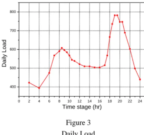
Figure 3 (February 3, 2003) represents the daily load curve. The values of the Load Scaling Factor (LSF) are given in Figure 4 with a maximum value of 1.35 for the maximum load of 782 MW.
0 2 4 6 8 10 12 14 16 18 20 22 24
400 500 600 700 800
Daily Load
Time stage (hr)
Figure 3 Daily Load
The coefficients of the transmission losses according to the powers generated for to the maximum load are:
01479 . 0 00137 . 0 00392 . 0
00137 . 0 01035 . 0 00052 . 0
00392 . 0 00052 . 0 00546 . 0
j
ai ,
0.03629
01680 . 0
02296 . 0 ) (
2
1
1 1 n
j i
Dj j aijP
bijQ , K0.1032
2 4 6 8 10 12 14 16 18 20 22 24
0.5 0.6 0.7 0.8 0.9 1.0 1.1 1.2 1.3 1.4
LSF
Hour
Figure 4 Load Scaling Factor
The cost functions [14, 15] providing the quantity of the fuel in Nm3/h necessary to the production are:
2000 150
85 . 0 )
(PGt1 PGt12 PGt1 F
850 75
4 . 0 )
(PGt3 PGt32 PGt3 F
3000 250
7 . 1 )
(PGt4 PGt42 PGt4 F
Under the constraints:
MW 510 30PGt1
MW 420 25PGt3
MW 70 10PGt4
ng
i
t L t D t W t
Gi P P P
P
1
0
4.2 Description of the Wind Farm
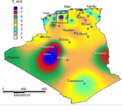
Figure 5 represents the map of the wind speed in Algeria to an altitude of 50 meters.
The map shows that the sites with the maximum wind speeds are those of Adrar (west south) and Tiaret (west north, in square) with a speed approaching 9 m/s and a recovered power density around 3.4 MWh/m2 [16].
The site of Tiaret is chosen for the implant of the wind farm. This one is supposed composed of 20 identical wind turbines with 40 meters blades.
Figure 5 Atlas of wind speed at 50 m
Due to a lack of data, we use the curve of variation of the wind speed of February 03, 2010 [17]. This curve, after interpolation, is represented by Figure 6. The variations of the power produced by the wind farm, the production of the thermal power plants and the total demand with respect to the time stage are illustrated in Figure 7.
0 2 4 6 8 10 12 14 16 18 20 22 24
2 4 6 8 10 12 14
Wind speed (m/s)
Time stage (hr)
Figure 6
Daily variation of the wind speed
0 2 4 6 8 10 12 14 16 18 20 22 24 0
100 200 300 400 500 600 700 800 900 1000
Load and Production (MW)
Hour
Total Demand Power plants production Wind farm production
Figure 7
Power production and Load demand
4.3 Carbon Dioxide Emission
For the combustion, the emission of carbon dioxide can be calculated with good precision from a balance of the carbon contained in the fuel. The Lower Heating Value or Net Calorific Value (NCV) and the content in carbon of the fuel, necessary to this calculation, can be measured accurately.
The calculation of carbon dioxide emissions related to energy use of fuels includes five steps [18]:
a) determination of the amount (ton) of fuel consumed during a time T, b) calculation of energy consumption from the quantity of fuel consumed and
the NCV of the fuel,
c) calculation of the potential carbon emissions from energy consumption and carbon emission factors,
d) calculation of actual carbon oxidized from oxidation factors (correction for incomplete combustion),
e) conversion of carbon oxidized to CO2 emissions.
Being of type H, The Algerian gas has the following characteristics:
995 0
5 15 78 0
6 49
3
. factor Oxidation
Kg/Gj . factor emission Carbon
Kg/m ρ .
Density
Gj/t . NCV
For determining the amount of fuel consumed in one hour, it is necessary to convert the flow from Nm3/h to m3/h. The law of boyle-mariotte-lussac permits us to write, to equal pressures:
) c (
/h m /h Nm
o
273 273
3 3
, (9)
which becomes for c°=20° : m3/h1.07Nm3/h
4.4 Results
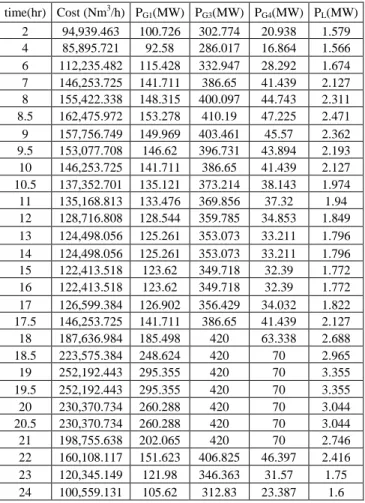
The simulations are realized by considering first the western Algerian electrical power system as it is (WA), then the western Algerian electrical power system with the injection of wind farm energy (WAW).The results of the production cost, for the two cases WA and WAW are shown in Figure 8 and detailed in Table 1 and Table 2.
Table 1 Production costs (WA case)
time(hr) Cost (Nm3/h) PG1(MW) PG3(MW) PG4(MW) PL(MW) 2 94,939.463 100.726 302.774 20.938 1.579 4 85,895.721 92.58 286.017 16.864 1.566 6 112,235.482 115.428 332.947 28.292 1.674 7 146,253.725 141.711 386.65 41.439 2.127 8 155,422.338 148.315 400.097 44.743 2.311 8.5 162,475.972 153.278 410.19 47.225 2.471 9 157,756.749 149.969 403.461 45.57 2.362 9.5 153,077.708 146.62 396.731 43.894 2.193 10 146,253.725 141.711 386.65 41.439 2.127 10.5 137,352.701 135.121 373.214 38.143 1.974 11 135,168.813 133.476 369.856 37.32 1.94 12 128,716.808 128.544 359.785 34.853 1.849 13 124,498.056 125.261 353.073 33.211 1.796 14 124,498.056 125.261 353.073 33.211 1.796 15 122,413.518 123.62 349.718 32.39 1.772 16 122,413.518 123.62 349.718 32.39 1.772 17 126,599.384 126.902 356.429 34.032 1.822 17.5 146,253.725 141.711 386.65 41.439 2.127 18 187,636.984 185.498 420 63.338 2.688 18.5 223,575.384 248.624 420 70 2.965 19 252,192.443 295.355 420 70 3.355 19.5 252,192.443 295.355 420 70 3.355 20 230,370.734 260.288 420 70 3.044 20.5 230,370.734 260.288 420 70 3.044 21 198,755.638 202.065 420 70 2.746 22 160,108.117 151.623 406.825 46.397 2.416 23 120,345.149 121.98 346.363 31.57 1.75 24 100,559.131 105.62 312.83 23.387 1.6
Table 2
Production costs (WAW case)
time (hr) Cost (Nm3/h) PG1 (MW) PG3 (MW) PG4 (MW) PL (MW) 2 93,215.571 99.216 299.611 20.183 1.583 4 84,590.505 91.388 283.516 16.268 1.57 6 111,322.561 114.708 331.364 27.932 1.713 7 145,207.921 140.956 385.077 41.061 2.124 8 154,346.252 147.56 398.523 44.364 2.306 8.5 161,377.042 152.522 408.616 46.846 2.465 9 156,673.062 149.213 401.887 45.191 2.357 9.5 151,277.129 145.345 394.076 43.256 2.186 10 143,467.912 139.7 382.443 40.429 2.017 10.5 133,250.207 132.06 366.826 36.61 1.967 11 129,473.321 129.183 360.897 35.17 1.932 12 118,527.727 120.626 343.25 30.888 1.845 13 115,399.179 118.095 338.103 29.622 1.796 14 116,274.976 118.796 339.566 29.973 1.796 15 115,067.226 117.809 337.576 29.48 1.773 16 116,755.205 119.159 340.396 30.156 1.773 17 122,287.385 123.562 349.453 32.359 1.82 17.5 142,393.989 138.913 380.818 40.038 2.115
18 183,848.594 180.017 420 60.595 2.746 18.5 217,686.873 238.179 420 70 3.01
19 243,833.352 282.314 420 70 3.374 19.5 241,981.121 279.362 420 70 3.38
20 219,244.474 240.974 420 70 3.122 20.5 216,679.09 236.358 420 70 3.142 21 185,327.934 182.175 420 61.669 2.938 22 152,910.221 146.592 396.35 43.877 2.38 23 116,654.701 119.059 340.258 30.107 1.751 24 98,790.598 104.11 309.667 22.631 1.603
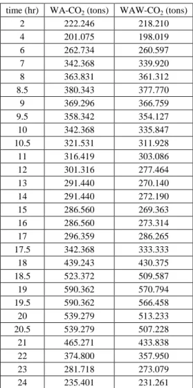
The total quantity of CO2 emitted is shown in Figure 9 and detailed in Table 3, while Figure 10 plots the CO2 emitted by every power plant.
The results show a difference between the costs of production and the CO2 emissions. The daily production cost for the WA case is around 4,338,332.219 Nm3/d and around 4,187,864.128 Nm3/d for the WAW case, which represents a difference of 150,468.091 Nm3/d.
0 2 4 6 8 10 12 14 16 18 20 22 24 80000
100000 120000 140000 160000 180000 200000 220000 240000 260000
Cost Nm3/h
Time stage (hr) Cost WAW Cost WA
Figure 8 Production Cost
0 2 4 6 8 10 12 14 16 18 20 22 24
150 200 250 300 350 400 450 500 550 600
CO2 emission (tons)
Time stage (hr) CO2 emission WAW CO2 emission WA
Figure 9 CO2 Emissions
0 2 4 6 8 10 12 14 16 18 20 22 24
0 50 100 150 200 250 300 350 400
CO2 emission (tons)
Time stage (hr) Power Plant 1 WAW Power Plant 2 WAW Power Plant 3 WAW Power Plant 1 WA Power Plant 2 WA Power Plant 3 WA
Figure 10
CO2 emissions by power plants
The daily CO2 emissions for the WA case are about 10,155.682 tons/d and around 9,803.448 tons/d for the WAW case, which represents a gain of 352.234 tons/d.
This gain is important considering that it is a winter day and therefore not very windy. Assuming that the wind has the same performance during a minimum of 80% of the year, the annual minimum amount of CO2 the atmosphere that can be saved is of the order of 103,000 tons.
Table 3 Detailed CO2 emissions
time (hr) WA-CO2 (tons) WAW-CO2 (tons)
2 222.246 218.210
4 201.075 198.019
6 262.734 260.597
7 342.368 339.920
8 363.831 361.312
8.5 380.343 377.770
9 369.296 366.759
9.5 358.342 354.127
10 342.368 335.847
10.5 321.531 311.928
11 316.419 303.086
12 301.316 277.464
13 291.440 270.140
14 291.440 272.190
15 286.560 269.363
16 286.560 273.314
17 296.359 286.265
17.5 342.368 333.333
18 439.243 430.375
18.5 523.372 509.587
19 590.362 570.794
19.5 590.362 566.458
20 539.279 513.233
20.5 539.279 507.228
21 465.271 433.838
22 374.800 357.950
23 281.718 273.079
24 235.401 231.261
Conclusion
In this paper, we study the effect of the injection of wind farm energy in the western Algerian electrical power system on cost and on the environment.
The dynamic environmental economic dispatch problem is solved via the Harmony Search Algorithm. The HSA is a meta-heuristic that uses a stochastic random search which is simple in concept, few in parameters and easy in implementation. Moreover, it does not require any derivative information.
The simulation results are very conclusive, since we showed that a minimum annual quantity of 103,000 tons of CO2 emissions can be restricted with a relatively small wind farm. Those emissions are equivalent to the emissions of more than 340,000 average vehicles of which the CO2 emission factor is equal to 0.2 kg/km [18] and traveling 1,500 km per year.
We recall here that the CO2 is a gas with notorious greenhouse effect and an average lifespan in the atmosphere of 100 years.
References
[ 1 ] Lu C. L., Chen C. L., Hwang D. S., Cheng Y. T.: Effects of Wind Energy Supplied by Independent Power Producers on the Generation Dispatch of Electric Power Utilities. Electrical Power and Energy Systems, Vol. 30 (2008) 553-561
[2] Wu J., Lin Y.: Economic Dispatch Including Wind Farm Power Injection.
Proceedings of ISES Solar World Congress: Solar and Human Settlement, (2007)
[3] Benasla L., Rahli M. : Optimisation des puissances actives par la méthode S.U.M.T avec minimisation des pertes de transmission. Second International Electrical Conference, Oran Algeria, 13-15 November (2000) [4] Boqiang R., Chuanwen J.: A Review on the Economic Dispatch and Risk
Management Considering Wind Power in the Power Market. Renewable and Sustainable Energy Reviews, Vol. 13 (2009), 2169-2174
[5] Lee K. S., Geem Z. W.: A New Meta-Heuristic Algorithm for Continuous Engineering Optimization: Harmony Search Theory and Practice. Comput.
Methods Appl. Mech. Engrg., Vol. 194 (2005) 3902-3933
[6] Robyns B., Davigny A., Saudemont C., Ansel A., Courtecuisse V., Francois B., Plumel S., Deuse J.: Impact de l’éolien sur le réseau de transport et la qualité de l’énergie. Proceedings of the Meeting of the Electro Club EEA, Competition in Electricity Markets, Gif-sur-Yvette, 15- 16 march (2006)
[7] Multon B., Roboam X., Dakyo B., Nichita C., Gergaud O., Ben Ahmed H. : Aérogénérateurs électriques. Techniques de l’ingénieur, D3960 (2004)
[8] Abdelli A.: Optimisation multicritère d’une chaîne éolienne passive. Ph.D.
thesis in electrical engineering from National Polytechnic Institute of Toulouse, October (2007)
[9] Wallach, Y., Even, R.: Calculations and Programs for Power Systems Network. Englewood Cliffs, Prentice-Hall (1986)
[10] Lukman D., Blackburn T. R.: Modified Algorithm of Load Flow Simulation for Loss Minimization in Power Systems. The Australian Universities Power Engineering Conferences (AUPEC’01) 23-26 September (2001)
[11] Elgerd O. I.: Electrical Energy Systems Theory. McGraw Hill Company (1971)
[12] Belmadani A., Benasla L., Rahli M.: A Fast Harmony Search Algorithm for Solving Economic Dispatch Problem. Przegląd Elektrotechniczny, 86 (2010) Nr. 3, 274-278
[13] Benasla L., Rahli M., Belmadani A., Benyahia M.: Etude d’un dispatching économique: application au réseau ouest algérien. ICES'06, Oum El Bouaghi, Algeria, 8-10 May (2006)
[14] Rahli M., Tamali M.: La répartition optimale des puissances actives du réseau ouest algérien par la programmation linéaire. Proceedings of the Second International Seminar on Energetic Physics, SIPE'2, Bechar, Algeria, November (1994) 19-24
[15] Rahli M., Benasla L., Tamali M.: Optimisation de la production de l’énergie active du réseau ouest algérien par la méthode SUMT.
Proceedings of the Third International Seminar on Energetic Physics, SIPE'3, Bechar, Algeria, November (1996) 149-153
[16] Kasbadji N. M.: Evaluation du gisement énergétique éolien contribution à la détermination du profil vertical de la vitesse du vent en Algérie. PhD thesis in physical energy and materials AbuBakr Belkaid University of Tlemcen, Algeria (2006)
[17] Observations, Previsions, Models in Real Time, www.metociel.com [18] Université Numérique Ing. & Tech.: The Thermodynamics Applied to
Energetic Systems. www.thermoptim.org
[19] CO2logic, Summary of the Study: Comparaison des émissions de CO2 par mode de transport en Région de Bruxelles-Capitale. conducted on behalf of STIB, January (2008)