Investigation of Residuated Monoids

(1)

Investigation of Residuated Monoids

S´andor Jenei

DSc dissertation

2011

(2)

.

(3)

Preface

Residuationis a basic concept in mathematics [11]. It is strongly connected with Galois maps [47] and closure operators. Residuated semigroups have been introduced in the 30s of the last century by Ward and Dilworth [113] to investigate ideal theory of commutative rings with unit.

The topic did not become a leading trend on its own right back then. In Hungary this concept goes back to Fuchs’ book [43] (see as well [106, 107] and [9]).

Nowadays the investigation ofresiduated lattices(that is, residuated monoids on lattices) has become quite popular, and has been staying in the focus of strong international attention. Several international conferences have been being devoted to this very topic, and several groups have been working on it from Japan via Europe to the United States. An extensive monograph discussing residuated lattices went to print in 2007 [46]. This increasing and significant interest was initiated by the discovery of the strong connection between residuated lattices and substructural logics [101, 100].

Substructural logics encompass among many others, classical logic, intuitionistic logic, rel- evance logics, many-valued logics, t-norm-based logics, linear logic and their non-commutative versions. These logics had different motivations, different methodology, and have mainly been investigated by isolated groups of researchers. The theory of substructural logics has put all these logics, along with many others, under the same motivational and methodological umbrella.

Residuated lattices themselves have been the key component in this remarkable unification. Ex- amples of residuated lattices include Boolean algebras, Heyting algebras [77], MV-algebras [21], basic logic algebras, [53] and lattice-ordered groups; a variety of other algebraic structures can be rendered as residuated lattices. Applications of substructural logics and residuated lattices span across proof theory, algebra, and computer science.

This dissertation deals with residuated semigroups. The related algebraic results often find applications in some related substructural logic. The dissertation consists of three main topics, namely, geometry, embedding, and structure.

Geometry

The main result of Chapter 1 is to characterize associativity of commutative, residuated operations by geometric notions, more precisely, with families of symmetries. Associativity of commutative operations is clearly equivalent to certain symmetries of the four-dimensional graph of the operation. Under a certain condition the trace of this four-dimensional symmetry becomes visible for the human eye as being families of certain three- and two-dimensional symmetries (called rotation-invariance in Section 1.3 and pseudo-inverses in Section 1.4, respectively). Even if this

7

(8)

condition fails to hold for the operation itself, it does hold for a particular quantic quotient of the operation. Moreover, transition from the operation to the quantic quotient can be understood in a geometric manner too. Thus, associativity of commutative residuated operations is visible for the human eye even if the condition in question does not hold. In addition, the main result of Section 1.5 is the discovery of another geometric property of residuated semigroups, called reflection-invariance. It is shown that under certain conditions, a subset of the graph of a commutative residuated chain (that is, a commutative, totally-ordered, residuated semigroup) is invariant under a geometric reflection. This result implies that a certain part of the graph of the semigroup operation determines another part of its graph via reflection on one hand, and tells us about the structure of continuity points of the monoidal operation (viewed as a two-place function) on the other.

This geometric understanding of associativity provides a kind of intuition such that certain algebraic relationships, such as the structure of involutive elements of an operation, or the equivalence between being naturally ordered and obeying a variant of the cancellation law, become understandable in a geometric way. In addition, this geometric intuition motivated an equivalent Hilbert-style axiom system for the logic IMTL in Section 1.7, and as well the introduction of the rotation and rotation-annihilation constructions in Chapter 7. By this geometric intuition one can, for example, give a purely geometric proof for the following statement: a semigroup operation on a partially ordered set with bottom is always a partially-ordered, residuated, integral monoid provided that the least element of the underlying universe in involutive. Last but not least, this geometric way of understanding algebraic notions has triggered the idea of solving an open problem on certain associative functions, posed by three leading experts of functional equations. It is quite remarkable that by applying this geometric approach, the usual method of reducing a problem in logic to an algebraic problem by tools of algebraic logic can sometimes be extended by a further reduction: an algebra to geometry reduction. In many cases the heuristic geometric proof of the related geometric problem can step by step be translated into an algebraic proof.

In Chapter 2 we present an applications of reflection-invariance and rotation-invariance for a long-studied problem in functional equations, namely, we apply it in the subdomain of uniqueness problem of associative functions [8, 79, 105, 16, 30, 109]. A subset of the domain of a function is called a subdomain of uniqueness if no two different functions from a given class of functions can be identical on that subset. T-norms are commutative, integral monoids on [0,1];

their left-continuity corresponds to being residuated. The questions of determining uniquely either a continuous Archimedean t-norm or a left-continuous t-norm on some vertical segments, on some horizontal segments, or on a narrow part of its domain are investigated. Remarkably, the continuous case (without assuming any further regularity conditions, such as, e. g., continuous differentiability) is the widest framework that can be addressed by tools of functional equations.

Continuity in algebraic terms is equivalent to being naturally ordered, which is a much smaller class than the residuated one. The fact that the residuated class can successfully be addressed by our geometric method (both in Chapter 2 and 3) shows its strength.

A conjecture of three leading experts of functional equations concerning the convex combi- nation of associative functions [6] is answered affirmatively in Chapter 3. It is shown that the nontrivial weighted arithmetic mean of two associative functions (from a certain class) is never associative provided one extra condition which can not be omitted. It is interesting to note that

(9)

CONTENTS 9 motivated by geometric insight the conjecture, which is originated in functional equations, has been reduced by using algebraic methods to a problem in real analysis about one-place functions, which has been solved by using integrals.

Embedding

In Chapter 4 we prove a conjecture of Esteva and Godo, namely, that the logicMTLis the logic of left-continuous t-norms. We prove it by showing that any countable linearly-ordered commutative residuated lattice can be embedded into a standard algebra, that is, where the monoidal operation is a left-continuous t-norm. This result is fundamental is three respects: First, it proves thatMTL is the most general t-norm-based logic, as opposed to the name ‘Basic Logic’ coined by H´ajek for his logic BL [53], which is the logic of continuous t-norms [19]. Second, this result paves the way for the discovery of the strong connection between t-norm-based logics and substructural logics [46, 88]. Third, the original embedding method of the proof has become important on its own right: Standard completeness of several other logics have been proved by slight modifica- tions of this embedding [25, 26, 37, 89]. Moreover, it has been shown that the existence of the Jenei-Montagna embedding is not only sufficient but as well necessary for the strong standard completeness of t-norm-based propositional logics [27]. In the second part of the section we show that this embedding method works for the non-commutative version ofMTLtoo.

Among the numerous construction methods introduced by Jenei, which result in left-continuous t-norms one is presented in Chapter 5. We shall construct via embedding a left-continuous t-norm from any countable, residuated, totally and densely ordered commutative integral monoid.

Moreover, we can construct a left-continuous t-norm from any countable, totally ordered, commutative integral monoid, which is not necessarily densely ordered and residuated. A special case, the embedding of such monoids over lexicographic product spaces is investigated in detail, and several examples are demonstrated.

Left-continuous t-norms are much more complicated than continuous ones, and obtaining a classification in the style of Mostert and Shields [90] seems to be a very hard task, if not impossible. In Chapter 6 we investigate some aspects of left-continuous t-norms, with emphasis on their continuity points. We prove that the set of continuity points of a left-continuous t-norm is a dense set and that the set of discontinuity points of a left-continuous t-norm is a zero measure first-category set. In particular, we are interested in left-continuous t-norms which are isomorphic to t-norms which are continuous in the rationals. We characterize such a class, and prove that it contains the class of all weakly cancellative left-continuous t-norms.

Structure

Jenei has generalized some of his construction methods from the[0,1]interval to the partially- ordered setting. The notion of involutive commutative residuated lattices will be generalized in Chapter 7 by introducing rotation-invariant semigroups. In addition, motivated by the geomet- rical characterization in Chapter 1, his rotation and rotation-annihilation constructions will be introduced and investigated, each of which can either be connected of disconnected. These constructions construct involutive residuated semigroups from residuated semigroups. The discon-

(10)

nected and connected rotation constructions have turned out to be fundamental in the structural description of perfect and bipartite IMTL-algebras [97], free nilpotent minimum algebras [13], free Glivenko MTL-algebras [24], and Nelson algebras [14], as well as in establishing a spectral duality for finitely generated nilpotent minimum algebras [15].

Motivated by reflection-invariance (in Chapter 1) we argue in Chapter 8 that the structural description of certain residuated operations inevitably requires the usage of the co-residuated setting. That is, residuation and co-residuation are not simply dual notions, such that it is sufficient to investigate only one of them, but rather notions complementing each another: They have to be considered simultaneously in certain settings, for instance, if the investigated operation is a commutative, densely-ordered, complete, residuated chain. A construction, called skew symmetrization, which generalizes the well-known cone-representation of ordered abelian groups will be introduced. Skew symmetrization uses both residuated and co-residuated operations simultaneously. It is shown that every commutative residuated monoid on a densely-ordered, complete chain with an involution defined by the residual complement with respect to the neutral element, and with the neutral element being the fixed point of the involution, can be characterized as the skew symmetrization of its underlying t-norm or its underlying t-conorm (t-conorms are the de Morgan duals of t-norms). This implies that the cones of the algebra (positive and negative ones) mutually determine one another.

By analogy with the cone representation of ordered Abelian groups, a construction – called symmetrization – is defined and it is related to the rotation construction in Chapter 9. Sym- metrization turns out to be a kind of dualized rotation, and accordingly, rotation turns out to be a kind of semi-symmetrization. Then a classification of those left-continuous t-norms is given for which their symmetrization is a commutative, residuated monoid.

Finally, yet another construction, called twin-rotation, will be introduced in Chapter 10. Twin- rotation generalizes symmetrization, and hence as well generalizes the well-known cone representation of ordered Abelian groups. It requires two operations on two cones and extends them to the union of the two cones. It will be shown that every conic commutative, involutive, residuated monoid can be represented as the twin-rotation of its cones. To have a closer look, we consider commutative, involutive, residuated monoids which are finite and linearly ordered. We are interested in which pairs of a positive and a negative cone result in commutative, involutive, residuated monoids via twin-rotation. On finite chains a critical notion is the “rank” which measures how the neutral element differs from the constant which is involved in the definition of the involution. We establish a one-to-one correspondence between positive and negative rank algebras, a connection which is somewhat similar to the well-known de Morgan duals. Finally, we give a classification of such algebras for the smallest and the largest possible non-positive ranks.

Each chapter is either self-contained or contains proper references to notions which are necessary to understand the content. Trying to keep some of the the chapters self-contained has sometimes resulted in a slight redundancy, mainly in the introductory parts. On the other hand, we hope it makes comprehension of the results easier.

(11)

Part I Geometry

11

(12)

(13)

Chapter 1 On the geometry of associativity

1.1 Introductory remarks

Abel considered associative functions in [1], which is arguably the first paper about semigroups [83]. He considers a real functionf such that the functionF(x, y, z) := f(z, f(x, y))is invariant under any permutation of the variables x, y, z. Abel calls such a function F (which is invariant under any permutation of variables) asymmetricfunction. This denotation implicitly refers to a connection between associativity and a kind of symmetry.

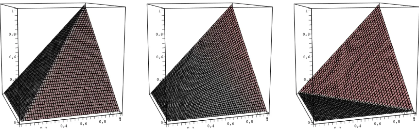
When considering binary operations on intervals of the real line, it is clear that their commutativity is readily seen from their graph. Associativity cannot be seen so easily. Figure 1.1 illustrates three commutative, associative binary operations on[0,1]; the minimum, the product, and the so-called Łukasiewicz t-norm¹, respectively. One can immediately see from the graphs

1 0,8

0,6 0,4

0,2 01 0,6 0,8

0 2 0,4 0 0,2 0,4 0,6 0,8 1

1 0,8

0,6 0,4

0,2 01 0,6 0,8

0 2 0,4 0 0,2 0,4 0,6 0,8 1

1 0,8

0,6 0,4

0,2 01 0,6 0,8

0 2 0,4 0 0,2 0,4 0,6 0,8 1

Figure 1.1: Minimum (left), product (center) and Łukasiewicz t-norms (right) the commutativity of these operations but not their associativity.

1The latter is given bymax(0, x+y−1); of course, we could use instead of this the simpler truncated addition x⊕y = min(1, x+y)but we prefer giving only conjunctive operations as illustrations, whereas the truncated addition is disjunctive. Other names for this operation are Calabbi mobbi’ ([56], p. 340) or ‘nilthread’.

13

(14)

1.1.1 Geometry of associativity in 4 dimensions

Following Abel we argue that associativity (together with commutativity) may be understood as a kind of symmetry in four-dimensional space. Indeed, consider the graph of a commutative, associative binary operation∗◦onXwhich is a subset ofX³defined by{(x, y, z)∈X³|z =x∗◦y}.

Commutativity of the operation is readily seen from the graph since it is equivalent to the invariance of the graph with respect to a reflection at the plane{(x, y, z)|x = y}. Unfortunately, no method is known for seeing the associativity of∗◦ in a similar manner. However, consider now {(x, y, z, v) ∈ X⁴ | v = (x∗◦y)∗◦z} and call it the four-dimensional graph of ∗◦. Associativity together with commutativity is clearly equivalent to the arguments of(x∗◦y)∗◦z being freely inter- changeable. This is equivalent to the four-dimensional graph being invariant with respect to three reflections at the hyperplanes, given by{(x, y, z, v)∈ X⁴ |x =y}, {(x, y, z, v) ∈X⁴ |y= z}, and{(x, y, z, v)∈X⁴|z =x}, respectively.

Our aim in this chapter is to develop a method for deciding associativity from the three- dimensional graph of an operation. Thus, a geometric characterization of associativity is presented here. This provides a deeper understanding of associativity, which turns out to be fruitful in conjecturing and proving algebraic results in the field of residuated lattices, and in establishing results in corresponding non-classical logics. Moreover, this geometric description has provided the intuition for a contribution to solving a long-standing open problem in the field of associative functions [65].

Throughout the section we illustrate our geometric characterization by computer generated pictures of surfaces in the unit cube or sections thereof. That is, we shall visualize our results by using linearly ordered semigroups [55] on the real interval[0,1].

Even though the visualization is possible only on compact intervals of R, all the results of the geometric characterization are true on partially-ordered sets too. The aim of the section is not only to introduce a kind of visualization aspect but, in addition, to understand algebraic relationships in a geometric manner. Visualization serves as a tool. It is interesting to notice that when conjecturing algebraic results based on geometric motivations, one can first heuristically prove them using geometry; then the steps of the geometric hint can step by step be translated into an algebraic proof.

1.2 Preliminaries

In the present section we shall consider residuated operations only. On intervals of R binary operations can be viewed as real functions of two variables, thus making it possible to talk about analytic properties in addition to algebraic ones. Several algebraic properties have analytic ana- logues in this setting. For example, being residuated corresponds to the left-continuity of such a two-place function.

(15)

1.2. PRELIMINARIES 15

1.2.1 Residuated groupoids

LetM be a nonempty set. An algebra(M,∗◦)is called a groupoid if ∗◦ is a binary operation on M. Thus we use the term ‘groupoid’ as is usual in universal algebra, which is different from what the same term means in category theory. A groupoid is calledcommutativeif∗◦is commutative.

Let(M,≤)be a poset. A mappingM →M is called aninvolutionif it is order-reversing and its composition with itself is the identity map ofM.

A groupoid on a poset (M,∗◦,≤) is called partially-ordered (po-groupoid) ifx∗◦y ≤ x∗◦z and y∗◦x ≤ z∗◦x whenevery ≤ z, (x, y, z ∈ M). When the underlying universe is a lattice, (M,∗◦,≤) is calledlattice-ordered (l-groupoid) if∗◦ is distributive over the join operation of the lattice. (M,∗◦,≤)is called residuated([9, 11, 43]), if there exist two binary operations →∗◦ and

∗

◦on it (called the left- and the right-residuum, or right- and left-adjoint, respectively) such that the following equivalences (called left- and right-residuation or left- and right-adjoint property, respectively) hold:

x∗◦y≤z if and only if x≤y→∗◦z (x, y, z ∈M) y∗◦x≤z if and only if x≤y ∗◦ z (x, y, z ∈M)

Equivalently,y→∗◦ z(resp. y ∗◦ z) is the largestx ∈M for whichx∗◦y≤ z (resp. y∗◦x ≤z) holds. When the groupoid is commutative, the two residua coincide, and will be denoted by

→_∗_◦. It is not difficult to see that residuated groupoids are partially-ordered; moreover, residuated groupoids are lattice-ordered if their underlying universe is a lattice [43, 57]. A po-groupoid will be calledconjunctiveifx∗◦y≤xandx∗◦y ≤y(x, y ∈M). A po-monoid is calledintegralif the unit element is the top element of the underlying poset. We say thatL=hL,≤,∗◦,→∗◦, ∗◦,1iis aresiduated latticeifhL,≤,1iis a lattice with top element1,hL,∗◦,1iis a monoid, and(L,∗◦,≤) is residuated with residua →∗◦ and ∗◦. A residuated lattice is commutative if so its monoidal operation. In this case we say that∗◦and→∗◦form a residuated pair.

1.2.2 Quantic quotients

Motivated by frame theory [77], which is of basic importance in the field of intuitionistic logic [45], the following terminology was introduced in quantal theory by Rosenthal [103]. Although all statements and terminology which are being recalled are about (not necessarily commutative) quantals there, they will be restated for the setting of commutative residuated groupoids and semigroups here (that is, we do not assume completeness of the underlying universe, but we do assume commutativity). The respective proofs from [103] could be repeated in this setting without any change.

Let(M,≤)be a poset andM= (M,∗◦,→∗◦)be a commutative residuated groupoid. A map- pingf :M →M is called aclosure operatorif it is an order-preserving, increasing, idempotent map. A closure operatorf is called aquantic nucleusif it satisfiesf(x)∗◦f(y)≤f(x∗◦y)for all x, y ∈M. Letf(M) ={f(x)|x∈M}.

Assume f is a quantic nucleus. Define a binary operation ? on f(M) by x ? y = f(x∗◦y).

ThenM_f = (f(M), ?,→_?) is a commutative residuated groupoid withx →_? y = f(x→∗◦ y),

(16)

and is called the quantic quotient ofMwith respect tof. Moreover, if∗◦is associative then so is

?.

A particular instance of quantic nuclei, which is of basic importance in this chapter, is the following. For an arbitraryc∈M define the maps¬^c : M →M and ^c : M →M by

¬^cx=x→∗◦c x^c=¬^c(¬^cx)

and call them thec-negation (other names arec-complementation orc-level function) and thec- closure operator, respectively. The graph of thec-level function is meant to be {(x,¬^cx) |x ∈ [0,1]}. An element which coincides with its c-closure is called c-closed. The operation ^c is a quantic nucleus (Proposition 3.3.4 in [103]).

The relation∼conM given by

x∼_c y if and only if x^c =y^c

is an equivalence relation and the equivalence class ofx ∈ M will be denoted by[x]_c. The pair (¬^c,¬^c)forms a Galois connection [47] between(M,≤)and(M,≤)and thus we have

¬^c(¬^c(¬^cx)) = ¬^cx. (1.1)

It follows from (1.1) that the set ofc-closed elements coincides with the range of the mapping¬^c. Note that the quantic quotient with respect to ^cis isomorphic to (and thus may be identified by) M_c= (M_c, ?,→_?), where

M_c = {[x]_c|x∈M} x ? y = [x^c∗◦y^c]_c x→_? y = [x^c→_∗_◦y^c]_c

We shall callMcthec-quotientofM.

If (M,∗◦,→_∗_◦) is a commutative, residuated semigroup, then for any c, x, y ∈ M the following statements hold: x≤ ¬^cy ⇐⇒ x^c≤ ¬^cy, and we havex∗◦y∼_cx^c∗◦y^c.

Proposition 1.1 In anyc-quotientM_cof any commutative residuated groupoidM, we have that[c]_cis the bottom element ofM_c, and the operation⁰ : M_c → M_cdefined by[x]_c⁰ = [¬^cx]_c for allx∈M is an order-reversing involution ofMc.

Proof. Straightforward verification.

Definition 1.1 Let(M,∗◦,≤) be a commutative residuated groupoid. An element c ∈ M is called involutiveif the mapping (of type M≥c → M) defined by x 7→ ¬^cx is an involution on M≥c = {x ∈ M | x ≥ c}. In other words, c ∈ M is called involutive if all the elements which are greater than or equal tocarec-closed.

(17)

1.3. GEOMETRY OF ASSOCIATIVITY IN 3 DIMENSIONS 17

1.3 Geometry of associativity in 3 dimensions

As we stated in Section 1.1.1 associativity of commutative operations can easily be seen in 4 dimensions. Our aim in the present section is not learning how things could be seen in 4- dimensional space but, more modestly, developing a method to visualize associativity of a commutative operation in 3 dimensions. In order to reach this goal, the intuitive idea of this section is to rewrite the original formulation of associativity(xy)z = x(yz) (∀x, y, z) in the following form first

(xy)z ≤c ⇔ x(yz)≤c (∀x, y, z, c), and then to rewrite it as follows (compare with (1.2))

xy ≤ c

z ⇔ yz ≤ c

x (∀x, y, z, c).

Therefore, the crucial definition will be the coming one:

Definition 1.2 (Algebraic Rotation Invariance Property)

Let(M,≤)be a poset and(M,∗◦,→∗◦)be a commutative residuated groupoid. Letc ∈ M. We say that∗◦isrotation-invariant with respect to¬^cif for allx, y, z∈M we have

x∗◦y≤ ¬^cz =⇒ z∗◦x≤ ¬^cy.

Observe that by applying it three times, rotation-invariance of∗◦with respect to¬^ccan be defined equivalently so that for allx, y, z ∈M we have

x∗◦y ≤ ¬^cz ⇐⇒ z∗◦x≤ ¬^cy ⇐⇒ y∗◦z ≤ ¬^cx. (1.2)

Proposition 1.2 Let (M,∗◦) be a commutative residuated groupoid. For any c ∈ M, the following statements are equivalent:

x∗◦y≤ ¬^cz ⇐⇒y∗◦z ≤ ¬^cx(⇐⇒z∗◦x≤ ¬^cy)holds 1. for allx, y, z,

2. for allc-closed elementsx, y, z.

If, in addition,∗◦is conjunctive then another equivalent formulation is:

3. for allx, y, z ≥c.

Proof. 1 =⇒ 3 and3 =⇒ 2are straightforward since c-closed elements are in[c,1]if ∗◦is conjunctive. To conclude the statement we shall prove2⇐⇒1. That is, we assume(x^c∗◦y^c≤ ¬^cz

⇐⇒y^c∗◦z^c ≤ ¬^cx)for all x, y, z, and we shall prove (x∗◦y ≤ ¬^cz ⇐⇒y∗◦z ≤ ¬^cx)for all x, y, z. By using the remark before Proposition 1.1, we havex∗◦y≤ ¬^cz⇐⇒x∗◦y^c≤ ¬^cz⇐⇒

x^c∗◦y^cc ≤ ¬^cz ⇐⇒x^c∗◦y^c ≤ ¬^cz, and similarly (y∗◦z ≤ ¬^cx⇐⇒y^c∗◦z^c ≤ ¬^cx). This ends the proof.

The following lemma plays a crucial role.

(18)

Lemma 1.3 (Rotation Invariance Lemma) Let (M,≤) be a poset and (M,∗◦,→_∗_◦) be a commutative residuated groupoid. The following two assertions are equivalent:

1. ∗◦is associative.

2. For allc∈M ∗◦is rotation-invariant with respect to¬^c.

Proof. Since in a poset the set of elements that are≥than a given element determines uniquely the element itself, associativity of∗◦is equivalent to the following:

(x∗◦y)∗◦z ≤c⇐⇒x∗◦(y∗◦z)≤c ∀c, x, y, z ∈M. (1.3) We have(x∗◦y)∗◦z ≤c⇐⇒x∗◦y≤ ¬^cz⇐⇒y∗◦z ≤ ¬^cx⇐⇒x∗◦(y∗◦z)≤c⇐⇒(x∗◦y)∗◦z ≤ c by the adjointness property, the rotation-invariance of ∗◦ with respect to ¬^c, the adjointness property together with commutativity, and the associativity of∗◦, respectively. Therefore, property (1.3), and thus associativity of∗◦is equivalent to the rotation-invariance of∗◦with respect to¬^cfor allc∈M. This ends the proof.

In the proof above the argument is somewhat similar to proving four equalities, say, a = b = c = d = a. Here if we do not assume e.g. b = c, then we can still infer it since we still have b =a=d =c. That is, if we do not assume1., but we assume2., then we can infer1., and vice versa.

1.3.1 The “straight line” case

In a commutative, residuated po-groupoid, the one-place function¬^cis an order-reversing map in general. However, in particular cases, its restriction to[c,1]can be an order-reversing involution of [c,1]. Keeping in mind that x 7→ 1−x is the standard order-reversing involution of [0,1], the denotation of the (algebraic) rotation-invariance property and the particular importance of the Rotation Invariance Lemma are explained by the following:

Lemma 1.4 (Geometric Interpretation I.)Let(M,≤)be a poset, and let ¬be aninvolution ofM. Define

σ : M³ →M³ given by

(x, y, z)7→(¬z, x,¬y). (1.4)

Then

1. σis a one-to-one mapping and its order is3, that isσ◦σ◦σ =id_M³.

2. The binary operation ∗◦ on M is “rotation-invariant with respect to ¬”, that is, x∗◦y ≤

¬z =⇒ z∗◦x≤ ¬y(∀x, y, z ∈M), if and only if the part of the spaceM³ which isabove the graph of∗◦remains invariant underσ.

3. Denoteρthe positive rotation of the unit cube[0,1]³by ^2π₃ which leaves points(0,0,1)and (1,1,0)fixed. If in addition,M = [0,1]with the usual ordering relation, and¬x = 1−x then

σ =ρ.

(19)

1.3. GEOMETRY OF ASSOCIATIVITY IN 3 DIMENSIONS 19 That is, if∗◦admits an (algebraic) rotation invariance with respect to¬, and the graph of x 7→ ¬xis a “straight line”, then the space above the graph of∗◦is invariant with respect toρ, which is a geometric rotation of[0,1]³. See Examples 1.6 and 1.8 later.

Proof. (σ◦σ◦σ)(x, y, z) = (σ◦σ)(¬z, x,¬y) = σ(y,¬z,¬x) = (x, y, z)by using the involutive nature of ¬. The space above the graph of∗◦is given byU ={(x, y, z)∈M³ |x∗◦y≤z}

which is equal to{(x, y, z)∈M³ |x∗◦y ≤ ¬(¬z)}. σ((x, y, z)) ∈ U means¬z∗◦x ≤ ¬y. Let u =¬z. Now, ifU is invariant underσ then it is clear thatx∗◦y ≤ ¬u =⇒ u∗◦x ≤ ¬yholds for allx, y, u∈ [0,1]since¬is onto. On the other hand, ifx∗◦y ≤ ¬u =⇒ u∗◦x≤ ¬yholds for allx, y, u∈[0,1], thenU is invariant underσ, by usingz =¬u.

The (positive) rotation of[0,1]×[0,1]×[−1,0]by ^2π₃ , which leaves the points(0,0,0)and (1,1,−1)fixed, is given as follows: It maps(1,0,0)to(0,0,−1),(0,1,0)to(1,0,0), and(0,0,1) to(0,−1,0). Therefore, being a linear operator, its matrix is given by

A=





0 1 0

0 0 −1

−1 0 0



,

and the of image each vector u =



 x y z



∈[0,1]×[0,1]×[−1,0]

under this linear operator isA·u. Denote the (positive) rotation of[0,1]³by ^2π₃ , which leaves the points(0,0,1)and(1,1,0)fixed byR. ThenRis given by

R(u) =A·



u−



 0 0 1







+



 0 0 1



.

Thus, the image of



 x y z



 under R is equal to





0 0 −1

1 0 0

0 −1 0



·







 x y z



−



 0 0 1







+



 0 0 1



 =





0 0 −1

1 0 0

0 −1 0



·



 x y z−1



+



 0 0 1



 =



 1−z

x

−y



+



 0 0 1



 =



 1−z

x 1−y



,

as easily verified. This concludes the proof of3.

Remark 1.5 Assume the hypothesis of Lemma 1.4.

The inverse ofσis given by(x, y, z)7→ (y,1−z,1−x), and is the (negative) rotation of [0,1]³ by ^2π₃ , which leaves the points(0,0,1)and(1,1,0)fixed.

Due to trichotomy, it may equivalently be said that∗◦is rotation-invariant with respect to¬ if and only if the part of the unit cube[0,1]³which isstrictlybelow the graph of∗◦remains invariant underσ.

(20)

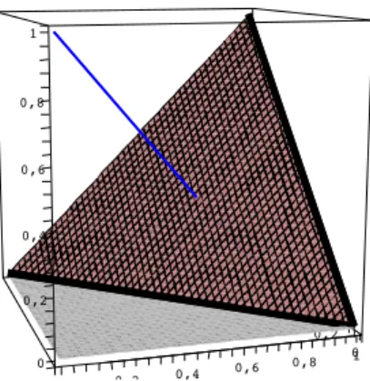
Example 1.6 Consider the Łukasiewicz t-norm (Fig. 1.1, right), that is,([0,1],∗◦,→_∗_◦), with x∗◦y= max(0, x+y−1),

x→∗◦y= min(1,1−(x−y)).

Since the Łukasiewicz t-norm is associative, it is rotation-invariant with respect to ¬^c for all c∈ [0,1]by the Rotation Invariance Lemma. In particular it is rotation-invariant with respect to

¬⁰. Moreover, we have ¬⁰x = 1−x, as is easily verified. We remark that from the definition of residuation, it is clear that the graph of¬⁰x can be seen from the plot: it is the border line in between the parts of the graph of∗◦where the value ofx∗◦yis0and>0, respectively. Lemma 1.4/3 is illustrated in Fig. 1.2.

10,8 0,60,4

0,2 0,8 01 0,4 0,6

0 2 0

0,2 0,4 0,6 0,8 1

Figure 1.2: The part of[0,1]³ which is above (or strictly below) the graph of∗◦is invariant with respect to the rotation of[0,1]³ by ^2π₃ around the axis. See Example 1.6

Remark 1.7 LetM = [0,1]. In complete analogy to Lemma 1.4, one can consider an involution¬on[c,1]for arbitraryc∈[0,1[, and defineσon[c,1]³in the same way. Thenσhas order 3 and if, in particular, the involution is equal tomin(1,1 +c−x), thenσis the (positive) rotation of [c,1]³by^2π₃ which leaves the points(c, c,1)and(1,1, c)fixed. Formulax∗◦y≤ ¬z ⇒ y∗◦z≤ ¬x (∀x, y, z ∈ [c,1]) means exactly that the part of the space[c,1]³ which is above the graph of∗◦ remains invariant underσ.

Example 1.8 As a by-product of the arguments in Remark 1.7, we get that associativity of the Łukasiewicz t-norm can immediately be seen from its graph. Indeed, by the Rotation Invariance Lemma, associativity is equivalent to the rotation-invariance of∗◦ with respect to¬^c for all c ∈ [0,1]. Again, it is clear that the graph of¬^c can be “seen” since it is the border line in between the parts of the graph of the Łukasiewicz t-norm, where the value of x ∗◦y is ≤ c and > c, respectively. But for all c ∈ [0,1], x ∈ [c,1], we have ¬^cx = 1 +c−x (a straight line) and therefore we only need to check that the part of the space[c,1]³ which is above (or strictly below) the graph of∗◦remains invariant under a rotation by 120^◦around the axis which goes through the points(c, c,1)and (1,1, c). Taking a look at Fig. 1.3, a moment’s reflection shows that it does hold, thus associativity of the Łukasiewicz t-norm is readily seen from its graph, as stated.

(21)

1.3. GEOMETRY OF ASSOCIATIVITY IN 3 DIMENSIONS 21

10,8 0,60,4

0,2 0,8 01 0,4 0,6

0 2 0

0,2 0,4 0,6 0,8 1

Figure 1.3: The part of[c,1]³(for anyc) which is above (or strictly below) the graph is invariant with respect to the rotation of[c,1]³ by ^2π₃ around the axis. See Example 1.8

1.3.2 The involutive case

How can we see associativity from the graph if the ¬^c’s are not “straight lines” but are only involutions?

DefineΦ = {ϕ|ϕis an order-preserving bijection from[0,1]to[0,1]}. It is easy to see that Φis the set of all continuous and strictly increasing functionsϕ : [0,1]→ [0,1]withϕ(0) = 0 and ϕ(1) = 1. The following theorem claims that each order-reversing involution of [0,1] is order-isomorphic to1−x.

Theorem 1.9 [110]Let ¬be an order-reversing involution of[0,1]. Then there existsϕ∈Φ such that forx∈[0,1]

¬x=ϕ⁻¹(1−ϕ(x)) = ϕ⁻¹◦(1−x)◦ϕ (x)

. Call ¬theϕ-transformation of1−x.

Of course we then have that1−xis theϕ⁻¹-transformation of¬. In a similar fashion, call∗◦ϕthe ϕ-transformation of∗◦if

x∗◦_ϕy=ϕ⁻¹(ϕ(x)∗◦ϕ(y)) (∀x, y, z ∈[0,1])

IfM = [0,1]and ¬ = ¬⁰ is an involution of [0,1], thenσ defined by (1.4) is a conjugate of a rotation of[0,1]³by an element ofΦ:

Lemma 1.10 (Geometric Interpretation II.)Let∗◦be a left-continuous t-norm, and assume that¬= ¬⁰is an involution of[0,1]. Letσbe as in (1.4), andρbe as in Lemma 1.4/3. Letϕ∈Φ such that theϕ-transformation of ¬⁰ is equal to1−x, and defineφ : [0,1]³ →[0,1]³by

φ(x, y, z) = (ϕ(x), ϕ(y), ϕ(z)).

Then

(22)

i. We have

σ=φ⁻¹◦ρ◦φ.

ii. The 0-level function of ∗◦_ϕ equals to 1 −x (and therefore the space above its graph is invariant with respect to the rotationρof[0,1]³.)

Proof. Indeed, such a ϕexists by Theorem 1.9, and the rest is verified by a straightforward computation as follows: We have¬⁰x=ϕ⁻¹(1−ϕ(x))forx∈[0,1].

(φ⁻¹◦ρ◦φ)(x, y, z) = (φ⁻¹◦ρ)(ϕ(x), ϕ(y), ϕ(z))

= φ⁻¹(1−ϕ(z), ϕ(x),1−ϕ(y))

= (ϕ⁻¹(1−ϕ(z)), ϕ⁻¹(ϕ(x)), ϕ⁻¹(1−ϕ(y)))

= (¬⁰z, x,¬⁰y)

= σ(x, y, z).

This provesi.

Denotingy =ϕ(x), we havex∗◦_ϕ(1−x) = 0if and only ifϕ⁻¹(ϕ(x)∗◦ϕ(1−x)) = 0if and only ifϕ(x)∗◦ϕ(1−x) = 0if and only ify∗◦ϕ(1−ϕ⁻¹(y)) = 0if and only ify∗◦ ¬y= 0, and the rest follows from the definition of residuation together with the strictly increasing nature ofϕ.

Clearly,ϕinduces an order-isomorphism between∗◦ϕ and∗◦. By virtue of Lemma 1.10/ii, when an operation has an involutive level function, from an algebraic viewpoint one can always think of it as if it were a “straight line”. Therefore, when formulating algebraic conjectures and trying to find a geometric hint for an algebraic proof, it is always enough to consider the “straight line”

case (Section 1.3.1, for which the geometric description is quite clear) rather than the involutive case (Section 1.3.2).

1.3.3 The general case

How can we see associativity from the graph if the ¬^c’s are not even involutions?

Proposition 1.11 Assume the hypothesis of Lemma 1.3, and let M_c be as in Section 1.2.2.

The following assertions are equivalent:

1. ∗◦is associative,

2. the?operation is associative inM_cfor allc∈M.

In other words,Mis a semigroup if and only if allc-quotients of it are semigroups.

3. For allc∈M the?operation inM_cis rotation-invariant with respect to the level function defined by the least element ofMc.

In other words,Mis a semigroup if and only if allc-quotients are rotation-invariant with respect to their level function defined by the least element.

(23)

1.4. GEOMETRY OF ASSOCIATIVITY IN 2 DIMENSIONS 23 Proof. 1.⇐⇒2. Associativity is inherited by quantic quotients as was mentioned in Sec- tion 1.2.2. To prove the other direction, assume, by contradiction, that there exists a c ∈ M such that the ? operation ofM_c is not associative. That is, there exist x, y, z ∈ M_c such that [x]_c?([y]_c?[z]_c) 6= ([x]_c?[y]_c)?[z]_c. M_cis isomorphic to the quantic quotient with respect to

cand hence we havex^c∗◦(y^c∗◦z^c)6= (x^c∗◦y^c)∗◦z^c, which contradicts the associativity of∗◦.

1.⇐⇒3. Assume ∗◦ is associative. Then, for any c ∈ M, M_c is a semigroup and hence by the Rotation Invariance Lemma the ? operation in M_c is rotation-invariant with respect to the level function defined by the least element of M_c. To prove the other direction, assume, by contradiction, that there exists x, y, z ∈ M such that (x∗◦y)∗◦ z = c 6= d = x∗◦ (y∗◦z).

Then we have either [c]_c 6= [d]_c or [c]_d 6= [d]_d. Indeed, if both were equalities then, by using basic properties of closure operators, we would haved ≤ d^c = c^c = c andc ≤ c^d = d^d = d, a contradiction. Hence we may safely assume [c]_c 6= [d]_c. Then the following holds in M_c: ([x]_c?[y]_c)?[z]_c= [c]_c6= [d]_c= [x]_c?([y]_c?[z]_c), which contradicts the associativity of?.

Remark 1.12 (Geometric Interpretation III.) It follows from Propositions 1.1 and 1.11 that the checking of the associativity of a commutative, residuated operation ∗◦ amounts to the verifying of the rotation-invariance property with respect to the involution defined by the least element in allc-quotients of it. In this way, using the notion of quantic quotients, the general case can be handled with the help of the involutive case:

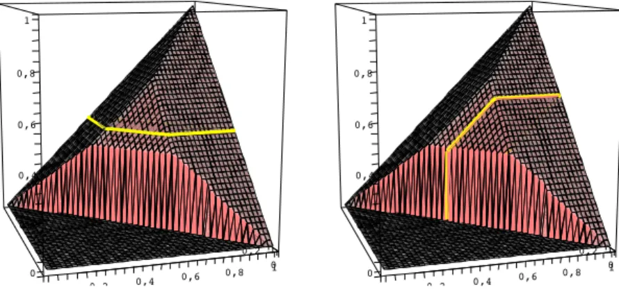
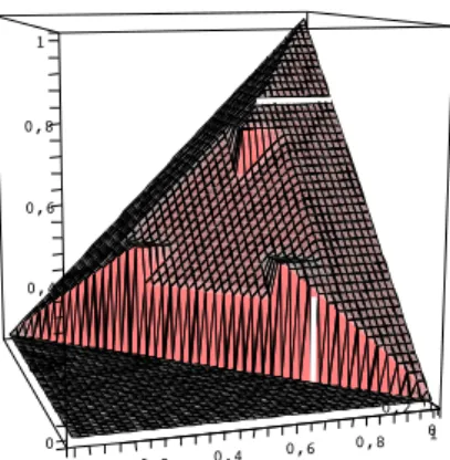
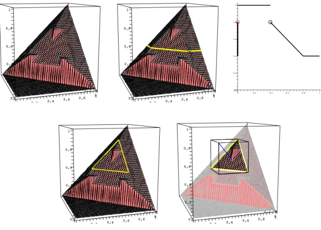
Example 1.13 Consider the operation which is depicted on the top-left of Fig 1.4. As an application of Section 1.3, we shall show that it is not associative.

Indeed, the horizontal cut of the graph at ²₅, and the ²₅-level function (that is, x →∗◦ 2 5) is depicted in Fig 1.4 (top-middle and top-right, respectively). Its range (that is the set of ²₅-closed elements) is ₂

5,⁴₅

∪ {1}. In the ²₅-quotient we have ₂

5

2 5

= [0,²₅] and [1]2 5

= [⁴₅,1]. Let us identify₂

5

2 5

by ²₅ and[1]²

5 by ⁴₅ in the ²₅-quotient. That is, in the sequel we shall consider the original operation restricted to₂

5,⁴₅

(bottom-left). By Proposition 1.11/3, this operation has to be rotation-invariant with respect to its least element, which is ²₅. But the ²₅-level function of the operation is a “straight line”, and therefore by Lemma 1.4 the (algebraic) rotation-invariance property in question has to appear as an invariance of its graph with respect to a real (geometric) rotation of ₂

5,⁴₅3

. Having a look at Fig. 1.4 (bottom-right), one can immediately see that is it not the case, whence the original operation is not associative.

1.4 Geometry of associativity in 2 dimensions

The aim of the present section is to point out that associativity of commutative operations can be seen even from the sectionsof the three-dimensional graph. Under sections we mean one-place functions of the form· ∗◦x, and¬^c., which aretwo-dimensionalobjects.

Definition 1.3 Define the pseudo-inverse of antitone mappings as follows: Let (M,0)be a poset with least element 0, and H be a poset. Further, letf : M → H be an antitone mapping

(24)

10,8 0,6

0,4 0,2

01 0,6 0,8

0 2 0,4 0

0,2 0,4 0,6 0,8 1

10,8 0,6

0,4 0,2

01 0,6 0,8

0 2 0,4 0

0,2 0,4 0,6 0,8 1

1

0,4 0,6 0,8

0,2 0,6

0,4

0,2

1 0

0,8

0

10,8 0,6

0,4 0,2

01 0,6 0,8

0 2 0,4 0

0,2 0,4 0,6 0,8 1

10,8 0,6

0,4 0,2

01 0,6 0,8

0 2 0,4 0

0,2 0,4 0,6 0,8 1

Figure 1.4: The operation, depicted on the top-left isnotassociative, see Example 1.13 such that for all y ∈ H, the least upper bound of the set {t ∈ M | f(t) ≥ y} exists inM. By declaringsup∅= 0, letf⁽⁻¹⁾ :H →M be a function defined by

f⁽⁻¹⁾(y) = sup{t∈M |f(t)≥y}.

Callf⁽⁻¹⁾the pseudo-inverse off. This definition is a particular case of a straight generalization of a concept (called quasi-inverse) for real functions [105, 70]. Iffis an order reversing bijection thenf⁽⁻¹⁾, of course, coincides with the usual inverse off.

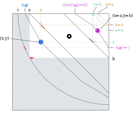
Remark 1.14 The notion of pseudo-inverses of monotone functions on intervals ofRhas a geometric interpretation: There is a simple geometric way to construct the graph of the pseudo- inversef⁽⁻¹⁾from the graph off [105].

i. Draw vertical line segments at discontinuities off.

ii. Reflect the graph off at the first median, i.e., at the graph of the identity function.

iii. Remove any vertical line segments from the reflected graph except for their upmost points.

(25)

1.4. GEOMETRY OF ASSOCIATIVITY IN 2 DIMENSIONS 25 The intuitive idea of this section is to characterize associativity by following equality (compare with (1.5))

c y

x = c xy. Therefore, the crucial definition of the section is

Definition 1.4 Let(M,≤)be a poset and letM= (M,∗◦,→∗◦)be a commutative residuated groupoid. We say that ∗◦ admits the pseudo-inverse property with respect to c ∈ M if for all x, y, z ∈M we have

x→∗◦¬^cy=¬^c(x∗◦y). (1.5)

Even though the pseudo-inverse property is an algebraic notion, it has a strong connection to pseudo-inverses of monotone functions as we shall shortly see. For anyc∈M, we have that the rotation invariance property with respect to¬^cand the pseudo-inverse property with respect toc are equivalent under the assumption of commutativity. Moreover, those are equivalent to a kind of symmetry of certain one-place mappings. The next statement extends the Rotation Invariance Lemma and thus provides other characterizations for the associativity of commutative operations.

Lemma 1.15 (Pseudo-Inverse Property Lemma)Assume the hypothesis of Lemma 1.3. Let c∈M. The following statements are equivalent:

1. ∗◦is rotation-invariant with respect to¬^c,

2. ∗◦has the pseudo-inverse property with respect toc,

3. For anyx∈M, thec-complement of the vertical section of∗◦atxdefined byf_x :M →M, y7→ ¬^c(x∗◦y)

is the pseudo-inverse of itself.

Proof. First we shall prove the equivalence between1and2. By residuation,x∗◦y≤ ¬^czholds if and only ifx→∗◦¬^cz ≥y. By the pseudo-inverse property, it is equivalent to¬^c(x∗◦z)≥y. This is equivalent tox∗◦z ≤ ¬^cyby using adjointness, commutativity, and adjointness, respectively, and it is equivalent toz ∗◦x ≤ ¬^cyby commutativity. Finally, it is equivalent tox∗◦y ≤ ¬^cz by the rotation-invariance of∗◦. This ends the proof².

Next, we prove the equivalence between2and3. It is straightforward to see thatf_xis antitone.

We claim that least upper bound of {t ∈ M | f_x(t) ≥ y} exists for all x, y ∈ M. Indeed, {t∈M |f_x(t)≥y}={t∈M | ¬^c(x∗◦t)≥y}={t∈M |x∗◦t≤ ¬^cy}, and the supremum of this set exists sinceM is residuated and the supremum is the existing greatest element of the set.

We havef_x(y) =¬^c(x∗◦y) = x→_∗_◦¬^cy= sup{t∈M |x∗◦t≤ ¬^cy}= sup{t ∈M| ¬^c(x∗◦t)≥ y}= sup{t ∈M |f(t)≥y}, again, if and only if the pseudo-inverse property holds.

2See the remark after the proof of Lemma 1.3.

(26)

That is, the pseudo-inverse property admits the following geometric interpretation: Let M be linearly ordered, e.g., M = [0,1]. Lemma 1.15 shows that for any x, c ∈ [0,1] the graph of v_x,c : [0,1] → [0,1], y 7→ ¬^c(x∗◦y) has the following geometric property: First, extend its discontinuities with vertical line segments. Then the graph obtained is invariant under the reflection at the line given byy =x.

The case when the easiest to see the geometric property above is if ¬^cis a kind of involution of[c,1], which is a “straight line”, that is, when¬^cx = 1 +c−x, x ∈ [c,1]. Then the vertical section y 7→ x ∗◦y (y ∈ [c,1]) itself has a symmetry property. The second row of Figure 1.5 illustrates this case.

1 0,8

0,6 0,4

0,2 01 0,6 0,8

0 2 0,4 0 0,2 0,4 0,6 0,8 1

1 0,8

0,6 0,4

0,2 01 0,6 0,8

0 2 0,4 0

0,2 0,4 0,6 0,8 1

1 0,8

0,6 0,4

0,2 01 0,6 0,8

0 2 0,4 0

0,2 0,4 0,6 0,8 1

Figure 1.5: Graphs of monoids on[0,1]and their vertical cuts at0.5

Geometric Motivation for Lemma 1.15/1=⇒3.

Horizontal cuts of the graph of ∗◦are curves that are symmetric in the sense of Remark 1.14 due to commutativity of∗◦. Assume ¬⁰x = 1−x, and assume that∗◦ is rotation invariant with respect to¬⁰. The image of a horizontal cut under ρ(defined in Lemma 1.4) is part of a partial mapping. Sinceσmaps symmetric curves into symmetric curves, the kind of symmetry which is described in Lemma 1.14 is preserved for the partial mappings. Thus,f_x :M →M,y7→1−x∗◦y is the pseudo-inverse of itself (see Fig. 1.6).

(27)

1.5. REFLECTION INVARIANCE OF RESIDUATED CHAINS 27

10,8 0,6

0,4 0,2

01 0,6 0,8

0 2 0,4 0

0,2 0,4 0,6 0,8 1

10,8 0,6

0,4 0,2

01 0,6 0,8

0 2 0,4 0

0,2 0,4 0,6 0,8 1

Figure 1.6: The symmetry of the horizontal cut is inherited by the vertical cut, being its image under rotation. See “Geometric Motivation for Lemma 1.15/1=⇒3” before Section 1.6

1.5 Reflection invariance of residuated chains

Proposition 1.16 Let(X,∗◦,→∗◦,≤)be a commutative residuated semigroup on a poset.

1. Forx, a∈X we have(x→∗◦a)→∗◦a ≥x.

2. The following statements are equivalent:

(a) xisa-closed,

(b) for everyx₁ > xwe havex₁→∗◦a < x→∗◦a.

Proof. By residuation,(x→∗◦a)→∗◦a≥xis equivalent tox∗◦(x→∗◦a)≤a, which is equivalent tox→_∗_◦a ≥x→_∗_◦a. This proves1. To prove the equivalence in the second statement assumex isa-closed andx₁ > x. By the antitone property of→∗◦ in its first component we havex→∗◦a≥ x₁→∗◦a. Ifx→∗◦awere equal tox₁→∗◦a, then it would lead tox= (x→∗◦a)→∗◦a = (x₁→∗◦a)→∗◦

a≥x₁, a contradiction. This proves2a⇒2b. Ifxis nota-closed then we have(x→_∗_◦a)→_∗_◦a > x by1. Lettingx₁ = (x→∗◦a)→∗◦aand referring to((x→∗◦a)→∗◦a)→∗◦a=x→∗◦awhich holds for all residuated semigroups, we obtain x₁ →∗◦ a = x→∗◦ a, a contradiction to2b. Hence the proof of2b⇒2ais concluded.

Definition 1.5 For a commutative residuated posetX = hX,≤,∗◦,→∗◦,1iand for x, y ∈ X define

x∗◦_coy =











inf{x₁∗◦y₁ |x₁ > x, y₁ > y} if neitherxnoryequals the top element ofX (if any) inf{x₁∗◦y|x₁ > x} ifyequals the top element ofX

inf{x∗◦y₁ |y₁ > y} ifxequals the top element ofX

x∗◦y if bothxandycoincide with the top element ofX if the infimum exists. Observe that incompleteposets∗◦_cois a binary operation since the infimum always exists.

(28)

(?) In addition, assume X is acompleteand densely-ordered chain. Thenx∗◦_coy = x∗◦y iff (x, y)is a continuity point of∗◦ (viewed as a two-place function) in the order topology of the chain. Then for∗◦being residuated is known to be equivalent to being left-continuous, as a two-place function (in the order topology) whereas being co-residuated is known to be equivalent to being right-continuous. By using that the chain is densely ordered together with that of the monotonicity of ∗◦, it is an easy exercise to prove that x∗◦_co y is equal to the limit ofx_i ∗◦y_i, x_i and y_i are being arbitrarily chosen sequences withx_i > x and y_i > y, converging to x andy, respectively. Call ∗◦_co the skewed modification of∗◦. It is right-continuous, by definition, therefore it is always a co-residuated operation, that is, it is residuated with respect to≥, the dual ordering relation ofL.

First, we state and prove thelocalversion of our main theorem on reflection-invariance.

Theorem 1.17 (local reflection-invariance)LetX = (X,∗◦,→∗◦,≤)be a commutative residuated semigroup on a complete chain. Leta, b, c∈Xbe such thata=b→∗◦c. Let(x, y)∈X×X be such thatx∗◦y=x∗◦coyand any of the following three set of conditions is satisfied:

1. (a) Neitherxnoryequals the top element of the chain (if any), (b) xisa-closed, andyisb-closed,

(c) sup{t→∗◦c|t > x∗◦y}=x∗◦y→∗◦ c.

2. (a) Exactly one ofxandy(sayy) equals the top element of the chain, (b) xisa-closed, andy∗◦(y→_∗_◦b) = b,

(c) sup{t→∗◦c|t > x∗◦y}=x∗◦y→∗◦ c.

3. Bothxandyequal to the top element of the lattice, which is the neutral element of∗◦, and a∗◦b=c.

Then

(x→∗◦a)∗◦(y→∗◦b) = x∗◦y→∗◦c. (1.6) Proof. Note that ∗◦_co is an operation on X since the chain is complete. We have [x∗◦y] ∗◦ [(x→∗◦a)∗◦(y→∗◦b)] = [y∗◦(y→∗◦b)]∗◦[x∗◦(x→∗◦a)] ≤ b∗◦a = b∗◦(b→∗◦c) ≤ c,and hence (x→∗◦a)∗◦(y→∗◦b)≤x∗◦y→∗◦cholds.

Assume that condition set1. holds. First we state

(x→∗◦a)∗◦(y→∗◦b)> x₁∗◦y₁ →∗◦c for x₁ > x, y₁ > y, (1.7) which is equivalent to [x₁∗◦y₁]∗◦[(x→∗◦a)∗◦(y→∗◦ b)] > c for x₁ > x, y₁ > y, sinceX is a chain. Sincexis a-closedx→∗◦ a > x₁ →∗◦a follows from Proposition 1.16, and analogously, y→∗◦ b > y1 →∗◦ b. Therefore x1 ∗◦(x→∗◦a) > a and y1 ∗◦(y→∗◦b) > b since X is a chain.