Classi fi cation of minerals and the assessment of lithium and beryllium content in granitoid rocks by laser-induced breakdown spectroscopy
Patrick Janovszky,abKriszti´an Jancsek,cD´avid J. Pal´asti,abJudit Kopniczky,d B´ela Hopp, bdTivadar M. T ´oth cand G´abor Galb´acs *ab
This study demonstrates that LIBS mapping and spatially resolved local analysis is an efficient and practical approach for the classification of mineral grains (quartz, feldspar, biotite, amphibole) and for prospecting of technologically relevant, low-Z elements (e.g. Be and Li) in granitoid rock samples. We tested three statistical approaches (classification tree (CT) based on indicator elements, linear discriminant analysis (LDA) and random forest (RF)) for the classification of the mineral grains and found that each of the three methods provides fairly similar, very good classification accuracies. RF and LDA provided better than 92%
accuracy for all minerals, whereas CT showed a somewhat poorer (around 80%) accuracy for quartz in particular. Our results also demonstrate that using multiple analytical locations within each grain and resting the classification on the majority vote of these individual analysis gives more reliable discrimination (grain-based accuracy is better than location-based accuracy). We also demonstrated that LIBS elemental mapping can provide valuable information about the distribution of chemical elements among the minerals, especially if it is combined with matrix-matched calibration of emission intensity data. We illustrated this by the successful assessment of ng tomg amounts of Be and Li in the studied mineral grains. Our results suggest that mining for Be and Li in granitoid rocks should be aiming for biotite and amphibole grains.
1. Introduction
As it is known, LIBS is a versatile, laser ablation-based atomic emission spectroscopy technique, which allows the fast and direct analysis of solid and liquid (even gaseous) samples with minimum sample preparation, in a non-contact, marginally destructive way.1–3Its routine conguration already makes trace (ppm level) elemental analysis possible for all elements of the periodic table, but more sophisticated laboratory setups (e.g.in double- or multi-pulse congurations) can even provide ppb- range detection limits.1,4Time-resolved analysis of the plasma emission also permits isotope-selectivity.5 There is ample demonstration in the literature that the feature-rich LIBS spectra can be successfully used for the accurate identication or discrimination of a variety of samples (chemical nger- printing).6–11Micrometer-resolution local analysis or elemental
mapping can also be done on solid samples, allowing for material science, medical, environmental or industrial appli- cations,1–3,9,12–14even in theeld.
One of the most appealing characteristics of LIBS is the possibility of direct solid sample analysis, which makes it of interest also to geologists and mineralogists. In this context, the analytical performance and package of attributes of LIBS have oen been compared to those of other spatially resolving solid sampling atomic spectroscopy techniques. Although it is not a perfect analytical technique, but LIBS does offer a uniquely advantageous combination of features. For example, laser ablation inductively coupled plasma mass spectrometry (LA- ICP-MS), which has several decades of success in geology, has a similar overall analytical potential, but is not portable, cannot be used in a stand-offconguration, struggles with the detec- tion of some lighter elements and has challenges in the quan- titative analysis due to issues related to the need for the transportation of ablated sample matter. Micro X-ray uores- cence spectrometry (m-XRF) is a popular desktop instrument in geochemical elemental analysis, but in contrast to LIBS it cannot sensitively detect low-Z elements (below Na), it has a narrower dynamic range, its spectra contain far less chemical information and it cannot be used remotely. Electron-probe micro analyzers (EPMA, similar to SEM-EDS or SEM-WDS) can provide very high spatial resolution and an elemental map
aDepartment of Inorganic and Analytical Chemistry, University of Szeged, D´om Square 7, 6720 Szeged, Hungary. E-mail: galbx@chem.u-szeged.hu
bDepartment of Materials Science, Interdisciplinary Excellence Centre, University of Szeged, Dugonics Square 13, 6720 Szeged, Hungary
cDepartment of Mineralogy, Geochemistry and Petrology, University of Szeged, Egyetem Street 2, 6720 Szeged, Hungary
dDepartment of Optics and Quantum Electronics, University of Szeged, D´om Square 9, 6720 Szeged, Hungary
Cite this:J. Anal. At. Spectrom., 2021, 36, 813
Received 27th January 2021 Accepted 18th March 2021 DOI: 10.1039/d1ja00032b rsc.li/jaas
JAAS
PAPER
within a very short time, but require tedious sample preparation and vacuum-ready samples and are very bulky and costly instruments. In addition they are not capable for measuring light elements or in theeld or stand-off, and have quite limited accuracy and dynamic range.1,15–17
Based on the above-discussed aspects, it is no wonder that LIBS is being increasingly explored by geologists and the mining and mineral processing industry in the last 10–15 years and is now more and more used for the analysis of geological material (GEOLIBS).15,16,18 A further, highly related, although more specialized application is planetary exploration using the LIBS instrumentation in the ChemCam system of the Curiosity Mars rover.9,19,20
LIBS geochemical analysis is generally directed towards one or the other of two primary and related goals: quantitative analysis of the elemental contents of rocks/minerals (e.g. ore prospecting) and identication of the minerals (e.g.mapping of geochemical and mineralogical footprints, provenance anal- ysis). For example, LIBS measurements with eld-applicable bespoke or laboratory-based instrumentation were success- fully demonstrated for the compositional analysis of silicate and carbonate minerals,21,22iron and phosphate ores,23–25spe- leothems,26,27monazite sand,28volcanic rocks,29,30soils,31uid inclusions32and other materials. In these studies, the concen- tration of several elements including Au, Fe, Cu, Zn, Pb, Ca, Mg, Sr, Mn, Si, Cr, Al, K, REEs,etc.were assessed by using principal components analysis (PCA), multivariate regression (PCR), articial neural network (ANN) analysis or partial least-squares regression (PLSR) for the construction of calibration models.
Either drill-core or ground rock samples were tested. In both cases, a large number of measurements are carried out to provide stratication or average concentration data.15,16,18 Another importanteld, where the on-site quantitative analysis of natural solid resources is needed and LIBS has already proven itself useful is the energy industry, more precisely coal analysis. For instance, the LIBS determination of carbon content, volatile content and the caloric value was shown to be practical and accurate enough33,34so that this information to be used for fuel type discrimination or control of coal-fueled power plants.
Mineral and rock type identication also necessitates the use of statistical data analysis. Broad discrimination of ore miner- alogy by PCA was demonstrated in selected wavelength windows in Australian iron ores.23Poˇr´ızkaet al.also used PCA to classify 27 igneous rock samples.35 In another study, PCA and so
independent modelling of class analogy (SIMCA) methods were used to generate a model and predict the type of samples.36 Harmonet al.used a spectral library approach to rapidly iden- tify and classify samples based on their dominant elements with a high degree of condence. It was observed that a maximum variance weighted – maximum correlation approach performs best. Minerals of different classes were correctly identied at a success rate of >95% for carbonates and
>85% for feldspars and pyroxenes.37 PCA and partial least squares discriminant analysis (PLS-DA) were used by Gottfried et al.38to identify the distinguishing characteristics of geolog- ical samples and to classify them based on their minor
impurities. The PLS-DA approach was later successfully extended to the provenance analysis of garnets,39 obsidian glasses,40 igneous and sedimentary rocks9 as well as conict minerals (e.g. columbite and tantalite).41 Most recently, the application of the advanced spectral angle mapper algorithm (SAM) for the identication of variations in the chemical composition in a complex chromite ore sample was also successfully demonstrated by Meima and Rammlmair.42 Nar- decchiaet al. introduced a new, LIBS-based spectral analysis strategy and named it embeddedk-means clustering, for the simultaneous detection of major and minor compounds and the generation of associated localization maps for the charac- terization of complex and heterogeneous rock samples at the micro-scale level.43
The above examples only illustrate the unique analytical potential of LIBS in geology-related or raw material exploration applications. This potential is expected to unfold in the coming years and more and more industrial, green-eld or brown-eld (mine), stand-off LIBS applications will be developed. This development is also propelled by the increased demand and declining reserves for raw materials needed by advanced tech- nologies. Two of the metals that are in high demand in recent years are Li and Be. Beryllium is widely used,e.g.in telecom- munications infrastructure, advanced medical diagnostics instrumentation, automobile components and aeroplane equipment. Lithium is also a greatly sought-aer metal, as it is used in large amounts in batteries, ceramics and glass, lubri- cating greases and polymer production. The uneven distribu- tion and limited availability made critical raw materials to be a subject of geopolitics and made the governments and companies44,45 realize that the mineral industry has to adopt new, cost-effective methodologies and technologies. LIBS is one of the promising andexible novel exploration tools, consid- ering its sensitivity towards all elements, speed, information- rich spectra, as well aseld- and stand-offapplicability.15
In the present study, we assess the potential of LIBS for the identication of minerals (biotite, feldspar, quartz and, partially, amphibole) and the distribution and quantitative amount of lithium and beryllium in granitoid rock samples.
The pros and cons of several analytical and data evaluation approaches are discussed and tested.
2. Experimental
2.1. Instrumentation
LIBS experiments were performed on a J-200 Tandem LA/LIBS instrument (Applied Spectra, USA), in the LIBS mode. This instrument is equipped with a 266 nm, 6 ns Nd:YAG laser source and a six-channel CCD spectrometer with a resolution of 0.07 nm. For every laser shot, the full LIBS spectra over the wavelength range of 190 to 1040 nm were recorded in the Axiom data acquisition soware, using a 0.5ms gate delay and 1 ms gate width. During the experiments, a 40mm laser spot size was maintained, as it allows for the sampling of sub- millimetre grains (small pieces of minerals making up a rock) at several locations, but is large enough to provide ample LIBS signal for trace element detection. The pulse
energy was generally set at 17.5 mJ and the laser repetition frequency was 10 Hz. The number of repeated measurements in one sampling location (without translation) was ten. The
rst shots were clean-up shots, so the spectra originating from them were discarded. Measurements were performed at 4–5 sampling points in each mineral grain (sampling was done in a total of 128 locations for biotite, 155 for feldspar, 83 for quartz and 4 for amphibole). LIBS experiments were carried out under argon, continuously rinsing the ablation cell with a gasow rate of 1 L min1. Argon gas increases the signal intensities and the continuousow decreases the fallout of ablation debris around at the crater.
Contact prolometry measurements performed on a Veco Dektak 8 Advanced Development Proler. The tip had a radius of curvature of 2.5 mm and the force applied to the surface during scanning was 30mN. The horizontal resolution was set to 0.267mm and 3.175mm in thexandyscan directions, respec- tively. The vertical resolution was 40A.
Optical images of the rock samples were taken with an Olympus BX-43 microscope equipped with an Olympus DP-73 camera, under polarised and transmitted light.
2.2. Materials
2.2.1. Samples. Three samples (M1, M2, M3) were taken from different locations within the M´or´agy Granite rock for the study. The main mass of the M´or´agy Hills belongs to the Eastern Mecsek Mountains of Hungary and consists of monzogranite, with monzonite inclusions crosscut by leucocratic dykes. At places, the igneous body has a foliated structure as it was affected by ductile deformation and metamorphic overprint.
The minor outcrop of the formation is known in the western part of the Mecsek as well. According to recent studies, the age of the formation is 310–320 million years according to K–Ar as well as zircon U–Pd geochronology.46 The rock types of the M´or´agy Granite Formation can be divided into four main groups: monzogranite (typical granitoid rocks); hybrid rocks;
monzonite (dark in colour and rich in magnesium and iron- bearing minerals) and leucocratic (light) dykes of different compositions. A continuous transition is induced by the hybrid rocks along the zone between the larger-sized monzonite realms and the host granitic rocks, which formed by the mixing of the two types of melt.46,47
Our studied samples are of the monzogranite type, i.e.
a granite variant with 35–65% feldspar. The fact that two different feldspars appear in the rock (orthoclase (K-rich) and plagioclase (Na-rich) feldspars) suggests that it had crystallized from magma saturated with water. Besides the two feldspars, the M´or´agy Granite contains the most common rock-forming minerals, quartz, biotite and, to a lesser extent, amphibole.
2.2.2. Standards.During the calibration and the examina- tion of matrix effects related to the minerals, various standards were employed. These included the NIST 610, 612 and 614 type glass reference materials, as well as biotite (biotite mica–Fe, from the massif of Saint-Sylvestre, France, provided by the Centre de Recherches P´etrographiques et G´eochimiques (CRPG)) and feldspar (JF-1 1985 Ohira feldspar Nagiso-machi,
Nagano Prefecture, Japan, provided by the Geological Survey of Japan (GSJ)) standards.
2.3. Methods
2.3.1. Sample preparation and reference mineral identi- cation.The rock samples were prepared for investigations in such a way that from each sample, a 30mm thin section was cut for mineral identication by optical microscopy and the remaining part of the bulk sample (originally in contact with the material of the thin section) was polished for LIBS analysis. This approach ensured that the rock surface submitted to LIBS analysis contained the same mineral grains which were identied.
The cutting was done using a diamond cutter (Struers Dis- coPlan) to form 35 20 10 mm rectangular bodies. These then underwent vacuum impregnation using ARALDITE AY103 and REN HY956 epoxy resins in a Struers CitoVac equipment.
Aer a full day of setting, a fresh surface was created on the impregnated rock body using the diamond cutter. The surface was ground using a Struers LaboPol-35 machine equipped with 80, 220, 500 and 1200 grit Struers MD-Piano diamond grinding wheels. As anal step, the aqueous suspension of SiC abrasive powder (Buehler) was applied to smoothen the sample surface.
30 mm thin sections of these rock bodies were cut using a Buehler PetroThin cutting and grinding machine. The thin sections were mounted on microscope slides using EpoFix epoxy resin. Aer 24 hours the samples were ready for optical microscopy. The mineral grains within the thin sections were identied and categorized under polarized light using optical microscopy, according to the standardized methods of petrology.48The remaining part of the prepared rock body (bulk) was used for the LIBS measurements.
A reasonable number of the four most common mineral grains in each sample were identied, labelled and numbered in the samples (Fig. 1). The total set of mineral grains in the three samples consisted of 33 biotite, 27 feldspar, 22 quartz grains and a single amphibole grain. Plagioclase and potassium feldspar grains were not distinguished.
2.4. Data evaluation
2.4.1. Random forest (RF).A random forest is a classier that consists of a collection of tree-structured classiers, where each decision tree, formed on random subset of variables, casts a vote for one of the input classes. The classication is based on their consensus. The prediction power of the RF is oen opti- mized by minimizing the so-called out-of-bag error (OOB error), which gives the percentage of false classications among the excluded subset of the training data. The two most important parameters of the random forest are the number of the trees grown, and the number of nodes in each tree. The OOB error usually declines with the increase of the number of trees, but the usage of too many trees it is not advisable as it would represent overtting. The node number indicates the splits, what every individual tree possesses; their number must be equal or larger thank1, wherekis the number of groups.49,50
2.4.2. Linear discriminant analysis (LDA). During linear discriminant analysis nobjects (spectra) are separated into k groups (samples) according to their m variables (spectral intensities). There are two different approaches to perform LDA, the so-called Bayesian and Fisher approaches, and the former one was applied in our study. The Bayesian approach assumes a multivariate normal distribution of every variables, and a prior probability (p1+p2+.+pn¼1) is assigned to every group. The posterior probability is calculated by using the equation below.
The group where an object belongs is selected based on the similarity of these posterior probabilities.51
Pði=xÞ ¼ fiðxÞpi
Pk
j¼1fjðxÞpj
2.4.3. Nelder–Mead simplex algorithm.The simplex algo- rithm is a geometry-based approach for function optimization.
It denes a scalable n + 1-point polygon (simplex) for the n- parameter function to be optimized and essentially moves this polygon across the response surface of the function. The func- tion isrst evaluated at each of the initial apex points of the polygon and it is established which is the edge of the polygon that is adjacent to the lowest values (for minimization). Then, the polygon is geometrically mirrored onto this edge and scaled up or down depending on how large the function value differ- ence was between the largest and smallest one in the preceeding simplex. This approach moves the polygon so that it zeroes in on the location of the extreme value of the function.52As with any function optimization, it is important also with the simplex method to have a good estimate for the initial coordinates of the polygon in order to avoidnding a local minimum instead of a global one.
Spectral line identication was carried out using version 18.0 of the built-in Clarity Soware (Applied Spectra, USA) of the LIBS instrument. Data processing was done mainly in the open- source RStudio Desktop soware package (v1.3),viadeveloping custom codes using the chemometrics, MASS, ALS, RPart and random forest modules of RStudio. The Nelder–Mead simplex
optimization algorithm was programmed and applied in MS Quick Basic programming language. The Image Lab soware (Epina, Austria) was used to visualize LIBS elemental maps, whereas the open access ImageJ soware was used to extract the surface area of mineral grains in microscopy images of the rock samples. The overall LIBS dataset submitted to RF and LDA contained as many as 12 288370¼4 546 560 data points.
3. Results and discussion
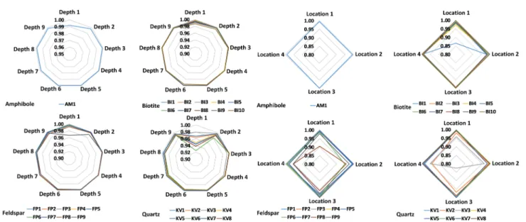
3.1. Compositional heterogeneities of the mineral grains Most mineral grains in igneous rocks grow during a longer time under various physical (rst of all pressure and temperature) circumstances and changing chemical conditions resulting in internal chemical zoning patterns. This is, from a chemical point of view, the manifestation of spatial changes of the composition inside a grain. The two most common types of zoning patterns are concentric and sector zoning, but other types, such as patchy, oscillatory, step and others also occur.53,54 These changes in chemical composition usually can be detected by different optical methods (e.g. Nomarski Differential Inter- ference Contrast (NDIC) microscopy, cathodoluminescence (CL),etc.), if the compositional changes also induce changes in the optical properties, or by scanning elemental mapping techniques (e.g.electron microprobe (EMP), secondary ion mass spectrometry (SIMS), proton microprobe (PIXE),etc.).53Minerals of magmatic rocks, such as the granitoid rocks studied here, are usually zoned. Although the lateral resolution (40mm) used in the present LIBS experiments is not capable to fully resolve zoning features of the smaller mineral grains investigated, the effect can still inuence the LIBS spectra collected at various locations and depths. Therefore, the extent of heterogeneity of the mineral grains in the samples was rst investigated by repeated measurements.
Individual LIBS spectra were collected from 10 shots deliv- ered at 4–5 locations within each mineral grain. LIBS data from therst shot (“cleaning shot”) were discarded and data from 9 depth levels were retained. Spectra within each mineral across locations or depths (intra-mineral variations) were then Fig. 1 Reflective optical microscopy images of the rock samples M1, M2 and M3 (M ´or´agy). The four studied mineral types are indicated in the images with abbreviations and borderline colours: AM¼amphibole (purple), BI¼biotite (orange), FP¼feldspar (green), KV¼quartz (blue).
Individual laser sampling locations are indicated by red dots.
compared to each other using the linear correlation function, which indicates full similarity with a Pearson correlation coef-
cient value of 1, and full dissimilarity with a value of 0 (assuming positive intensities).55,56Ray plots in Fig. 2 show the observed intra-mineral variations of each mineral grain in sample M1.
It was generally found that there is a reasonable similarity of spectra, indicated by correlation factors of at least 0.85 in most cases. It can also be seen that the inter-location (lateral) varia- tions, or heterogeneities, are signicantly larger than the inter- depth variations. This can be attributed to the larger spatial distance between locations (ca. 100–500 mm, cf. Fig. 1) than depth levels, which makes location-related changes from the same zone generally more observable. It is also apparent that the LIBS spectra from depth level 1 are quite dissimilar from the rest the depth-resolved data, hence the data not only therst (already discarded) but also from the second laser shot should be considered as a cleaning shot. Based on these observed variations, we decided that in the mineral classication part of our study, we use the depth-averaged LIBS spectra from depths 2–9 of each location in each mineral grain as a statistical data element.
Another observation made in data in Fig. 2 is that zoning in the present samples is most pronounced in quartz and feldspar grains, whereas variations between different grains of the same mineral are also clearly identiable. These observations should be considered when the accuracy of mineral grain classica- tions is evaluated in Section 3.3.
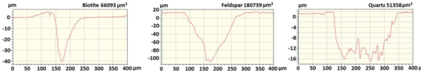
3.2. Laser ablation characteristics of the mineral grains The studied minerals are all silicates, but their generalized composition is disparate.53 Besides, their colours are also different, hence it can be expected that their laser ablation behaviours are different as well (because of the different light
absorption characteristics). To assess this, we investigated the laser ablation craters in the mineral grains by using contact prolometry aer delivering ten repeated laser shots under the same conditions as described in the Experimental section. The cross-sectional prolometry curves (Fig. 3) reveal that the crater depths and volumes are indeed highly different, which indi- cates that quantitative analysis (or certain discriminative anal- ysis) can only be attempted with reasonable accuracy if matrix- matched calibration or at least crater volume normalization (with a general silicate standard, such as the NIST 6XX glass series) is performed. The ablation depth per a laser shot was approximately 1.4mm for quartz, 4mm for biotite and 11mm for feldspar.
3.3. Qualitative discrimination of mineral grains
Considering the classication character of the analytical problem addressed here, we tested the performance of mainly multivariate chemometric methods (RF and LDA), which can also be called machine learning (ML) methods. In these methods, we used uncompressed data sets, as in our experi- ence, data compression oen leads to a distortion, which in turn may decrease the discrimination power and reliability (robustness) of the classication. This requires chemometric (or ML) methods that can cope with uncompressed data, which is the case with RF and LDA. In addition, we also assessed the performance of a more conventional approach in which the presence of spectral lines of indicator elements (characteristic of the mineral composition) were used for discrimination.
For model construction (training), we used minerals in sample M1. The model then was validated by using it on sample M2 and M3. The accuracy of the methods was established by comparing the predicted and actual mineral types; the accuracy was expressed in terms of correct classications. Moreover, we give calculated accuracy results according to two approaches:
Fig. 2 Intra-mineral compositional variations of each mineral grain in sample M1, as assessed by comparing LIBS spectra taken at various locations and depths by the linear correlation function. The average spectrum across the non-varying coordinate, depth or location, was taken as reference during the comparisons. The ray plots show the correlation coefficient on their radial axes.
a location- and a grain-based metric. The grain-based accuracy was obtained in the way that separate laser ablation locations (4–5 within each grains) were evaluated individually and the majority“vote”for the mineral type was associated with that grain. The location-based accuracy was calculated as the overall accuracy obtained when spectra from ablation locations in each grain were evaluated individually.
3.3.1. Classication by using indicative spectral lines.LIBS is a method of elemental analysis, thus one of the obvious potential approaches for the classication of mineral grains is to look for the presence of characteristic (indicative) spectral lines of the elements that make up the minerals. In the present case the nominal composition of the four minerals are [K(Mg,Fe)3(Al,Fe)Si3O10(OH,F)2] for biotite, [SiO2] for quartz, [NaAlSi3O8–KAlSi3O8–CaAl2Si2O8] for feldspar, and Na01Ca2(- Mg,Fe,Al)5(Al,Si)8O22(OH)2 for amphibole.53 Based on this knowledge, we have set up a simple protocol – essentially a controlled decision tree – for classication. The protocol, shown in Fig. 4, is based on the detection of characteristic major components Al, Fe, K and Caviathe presence or absence of their selected lines in the LIBS spectrum. Amphibole was actually not involved in this part of this evaluation, because the single grain studied of this mineral is not enough for a statisti- cally relevant evaluation–nevertheless we indicated its position in the decision tree structure.
For the testing of this protocol, the spectral lines of Al I 308.21 nm, Fe I 371.99 nm, Ca II 393.37 nm and K I 769.93 nm were selected from the NIST Atomic Spectra Database. Each of these spectral lines is free from interference, at the resolution of our LIBS instrument, from the other three elements, as well as from Si, O, Na and Mg, the other commonly occurring compo- nents of these minerals. It is essential for the functioning of the protocol that a given element is only considered as present if the intensity of its spectral line exceeds a threshold intensity cor- responding to a concentration level that classies as a major component (e.g. 0.5 m/m%). Corresponding intensity thresh- olds for the above four spectral lines were taken from calibra- tion plots obtained using the NIST glass (silicate) standards.
These four intensity thresholds were then used as initial esti- mates for the Nelder–Mead simplex optimization algorithm52 which was performed to maximize the accuracy of the classi- cation of all mineral grains in sample M1. As described earlier, depth-averaged LIBS spectra taken at each location in each grain were used as statistical elements in this classication.
When the simplex algorithm terminated, the optimized inten- sity thresholds were used to evaluate LIBS data from the mineral
grains in samples M2 and M3. A grain was only considered to be accurately identied if the majority of the locations within the grain gave correct identication. As can be seen, the classica- tion is very accurate for biotite and feldspar but is signicantly poorer for quartz, for which it is around 80% only. This result is in line with the formernding, namely that quartz grains are rather impure in the samples. The results also strongly suggest that sampling at several locations within each grain makes the identication more robust. Table 1 gives an overview of the accuracies obtained.
3.3.2. Classication by using random forests. Random forests (RF) is a multivariate method of classication, which can be considered to be the advanced version of the classication (or decision) tree approach. It was recently introduced by Brei- man in 2001.49The generally recognized advantages of the RF method includes the ability to work with large datasets (with Fig. 3 Ablation crater cross-sections of the mineral grains from ten repeated laser shots, as obtained by contact profilometry. The crater volume is indicated in the upper right corner of each graph.
Fig. 4 Flow chart for mineral grain classification based on the LIBS detection of major components Al, Fe, K and Ca.
thousands of variables), good accuracy and fast computation.
Random forests have recently been successfully used in LIBS sample discrimination studiese.g. on polymers,57 ceramics,58 steel samples59and iron ores.60
In the present application, we trained the RF with datasets on sample M1 and optimized the number of trees as well as the number of nodes. Up to 500 trees with up to 20 nodes were evaluated by monitoring the out-of-bag error. It was found that the OOB initially steeply decreases with the increase in the number of trees and asymptotically reaches its minimum at around 50. Simultaneously, the increase of the number of nodes clearly deteriorated the OOB; the minimum was found with as little as two nodes. All RF classication results were therefore obtained by using 100 trees with two nodes.
As can be seen in Table 1, RF gave good, well-balanced results. The accuracy for grain-based classication was at least 92.6% for all three minerals. Similarly to the indicator line approach, the grain-based accuracy (majority vote of sampling locations within the grain) was better than when classication by each sampling locations was considered. By scrutinizing the nodes, it is also possible to estimate the most important (most frequent) classiers. This analysis interestingly revealed that 274.29 nm, 400.84 nm, 345.65 nm and 326.08 nm were these
variables, which may be associated with Fe, Th and V, instead of major components of the rock-forming minerals.
3.3.3. Classication by using linear discriminant analysis.
Linear discriminant analysis (LDA), also known as discriminant function analysis, is a widely employed classication tech- nique.51It generally performs well in LIBS classication studies done on various samples, including rocks,10,34,61,62although it is known to give unstable results if multicollinearity is present in the data set.
We tested Bayesian LDA on our uncompressed LIBS data.
The results can be seen in Table 1 and Fig. 5. The overall clas- sication accuracy was good, over 87% based on separate sampling locations and over 92% for grains (based on the majority vote within a grain). False classications can be mostly associated with quartz and feldspar.
3.4. Quantitative assessment of the distribution of selected trace elements
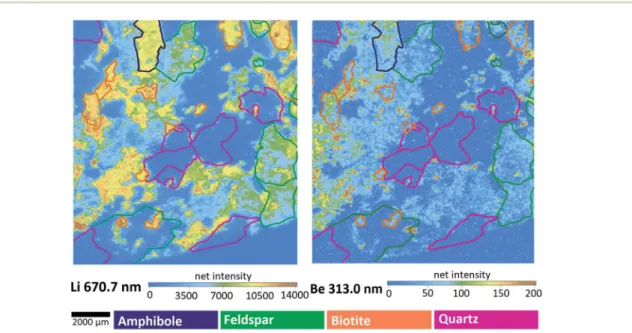
3.4.1. Mapping of Be and Li.Considering their relevance, we collected LIBS elemental maps of Be and Li in granitoid sample M1. Step scanning with non-overlapping laser spots (resolution: 40mm, laser pulse energy: 5 mJ) was employed in this part of the investigation. Spectral intensity-based elemental Table 1 The overall accuracy of the classification of minerals in all three rock samples according to the three employed statistical methods. The grain-based accuracy is based on the majority“vote”for the mineral type from all sampling locations within the grain. Location-based accuracy was calculated as the overall accuracy when spectra from ablation locations in each grain were evaluated individually
Indicator lines Random forest (RF) Linear discriminant analysis (LDA)
As per sampling
locations As per grains
As per sampling
locations As per grains
As per sampling
locations As per grains
Biotite 97.60% 100.00% 95.30% 97.00% 95.30% 97.00%
Feldspar 95.50% 100.00% 88.40% 92.60% 89.00% 92.60%
Quartz 80.70% 77.30% 84.30% 95.40% 87.90% 95.40%
Fig. 5 Biplot of the LDA classification results of the mineral grains.
maps for Be II 313.0 nm and Li I 670.7 nm lines can be seen in Fig. 6. Besides other uses proposed recently in the literature for such LIBS elemental maps, such as grain boundary42or grain size determination,63here we demonstrate that it is possible to identify the type of mineral that contains most of the targeted trace elements. By the comparison of Fig. 6 and 1, it can be realized that biotite and amphibole grains contain the most Li and Be, whereas feldspar has signicantly lower amounts of both elements. As Li+has a cation radius rather close to that of Mg2+, in most crystal lattices Li incorporates to the position occupied by Mg. Among the studied phases, biotite and amphibole are the minerals where the Mg4 Li exchange is possible. Similarly, due to the close geochemical behaviour of [BeO4]6 with [AlO4]5, beryllium can replace aluminum in most silicate structures, like in the feldspar and mica (biotite) lattices. As there is no exchangeable cation in its structure, not surprisingly, quartz has the least traces of these metals. The distribution of Be and Li among the grains seem to be quali- tatively correlated. These results suggest that mining for Be and Li in granitoid rocks should be aiming for biotite and amphi- bole grains. A promising approach for such a mining activity may be the ISL (in situ leaching) technique, which is being intensively developed recently.64
3.4.2. Quantitative estimation of the Be and Li content.
Intensity-based elemental maps provide limited information for prospecting purposes, therefore we also performed calculations to quantitatively assess the Be and Li content in the mineral grains of samples M1 to M3 (only considering those biotite, feldspar and quartz grains which were identied in Fig. 1.). Net intensity data for the Li I 670.7 nm and Be II 313.0 nm spectral lines collected at the measurement locations indicated in Fig. 1 were converted to concentrations by calibration using matrix- matched standards. The NIST 612 standard was used for quartz calibration based on their similar laser ablation behav- iour (similar crater volumes). The average of the 4–5
concentration data obtained within each grain was assigned to that grain and then the surface area of the grain, determined by the ImageJ soware, and the typical density value of the mineral was used to convert this to the mass of Be and Li present in each grain. We assumed an arbitrary, uniform 100mm“depth”value during the volume determination; this value is roughly the average grain diameter in our sectioned samples – a better estimation for the individual grain volumes was not available.
The results are summarized in Fig. 7 and reveal that ng tomg amounts of the metals could be quantitatively determined by LIBS. On the le panel of the gure the metal contents expressed in mass, and on the right panel in concentration, can be observed.
Data in Fig. 7 justify the assumption suggested by the intensity-based elemental maps namely that the Li and Be content varies concertedly in all three minerals – the pattern show that generally (with very rare exceptions) wherever the Li content is high, so is the Be content. The mass of the metals present in the grains naturally changes with the size of the grain, thus the concentration distribution does not follow the same pattern, but the relative contents of Be and Li follow the same trend. Be concentrations (amounts) are in the same magnitude as Li concentrations (amounts) in quartz and feld- spar, whereas they are signicantly different in biotite, in which Li concentrations are almost one hundred times higher than those of Be. Not surprisingly, quartz contains the smallest amounts of both metals. It is also apparent that feldspar is the best source of Be, whereas biotite is for Li. According to the relevant report published by the Geological Institute of Hun- gary, the mineral composition of M´or´agy Granite samples is 10% biotite, 70% feldspar and 15% quartz, with the remaining 5% being mostly amphibole.65 Using this average mineral composition data, an estimate can be given for the overall Be and Li content of these rocks: 1 kg of these rocks containca.
28 mg of Be and 144 mg of Li.
Fig. 6 Intensity-based step-scan LIBS elemental maps of the M1 sample. Colors of the contours are indicating the mineral types, as seen in Fig. 1.
4. Conclusions
We have shown that LIBS mapping and spatially resolved local analysis is an efficient and practical approach for the classi- cation of mineral grains (quartz, feldspar, biotite, amphibole) and for prospecting of technologically relevant elements in granitoid rock samples. We have tested three statistical approaches for the classication and it was demonstrated that better than 92% classication accuracy is achievable by using random forests and linear discriminant analysis. Direct classi-
cation by assessing the presence of the characteristic elements (decision tree based on indicative spectral lines) is a powerful method but can lead to great failure rates in case of relatively pure minerals, such as quartz. Our results also revealed that using multiple analytical locations within each grain and resting the classication on the majority vote of these individual analysis gives more reliable discrimination. We also demon- strated that LIBS elemental mapping can provide valuable
information about the distribution of chemical elements in the minerals, especially if it is combined with the matrix-matched calibration of emission intensity data.
It is also worth emphasizing that the appeals of LIBS in this and similar geochemical and mining industry-oriented appli- cations include that it is a highly versatile analytical technique which is portable, robust, can be used in a stand-offsituation and is equally sensitive to light and heavy elements. This is a unique set of features among atomic spectroscopy techniques.
In our opinion, the sensitivity of the technique is well demon- strated by the fact that we successfully assessed ng to mg amounts of Be and Li in the studied mineral grains. We also point out that the described LIBS analytical and data evaluation approaches can be potentially fairly easily generalized and automated. For example, once grain boundaries in a rock sample are automatically identied by modern computer vision and machine learning methods (e.g.ref. 42), spatially resolved LIBS analysis can identify the mineral types and use this Fig. 7 The Li and Be content of each analyzed mineral grain, expressed in terms of mass (on the left) and ppm concentration (on the right).
information to select the proper calibration standards (cali- bration curves) that can be used to convert spectral intensity data to concentration (mass) data of relevant elements.
Con fl icts of interest
There are no conicts to declare.
Acknowledgements
Thenancial support received from various sources including the Ministry of Innovation and Technology (through project no.
TUDFO/47138-1/2019-ITM FIKP and T´emater¨uleti Kiv´al´os´agi Program TKP 2020) and the National Research, Development and Innovation Office (through projects no. K_129063, EFOP- 3.6.2-16-2017-00005 and GINOP-2.3.3-15-2016-00040) of Hun- gary is kindly acknowledged.
References
1 G. Galb´acs,Anal. Bioanal. Chem., 2015,407, 7537–7562.
2 F. J. Fortes, J. Moros, P. Lucena, L. M. Cabalin and J. J. Laserna,Anal. Chem., 2013,85, 640–669.
3 D. W. Hahn and N. Omenetto,Appl. Spectrosc., 2012,66, 347–
419.
4 N. Jedlinszki and G. Galb´acs,Microchem. J., 2011,97, 255–
263.
5 A. Bol'shakov, X. Mao, J. J. Gonz´alez and R. E. Russo,J. Anal.
At. Spectrom., 2016,31, 119–134.
6 A. Metzinger, R. Rajk´o and G. Galb´acs,Spectrochim. Acta, Part B, 2014,94, 48–57.
7 J. Moros, J. Serrano, C. Sanchez, J. Macias and J. J. Laserna,J.
Anal. At. Spectrom., 2012,27, 2111–2122.
8 S. Manzoor, S. Moncayo, F. Navarro-Villoslada, J. A. Ayala, R. Izquierdo-Hornillos, F. J. Manuel de Villena and J. O. Caceres,Talanta, 2013,121, 65–70.
9 A. M. Ollila, J. Lasue, H. E. Newsom, R. A. Multari, R. C. Wiens and S. M. Clegg,Appl. Opt., 2012,51, B130–B142.
10 D. J. Pal´asti, A. Metzinger, T. Ajtai, Z. Boz´oki, B. Hopp,
´E. Kov´acs-Sz´eles and G. Galb´acs, Spectrochim. Acta, Part B, 2019,153, 34–41.
11 G. Vitkova, K. Novotny, L. Prokes, A. Hrdlicka, J. Kaiser, J. Novotny, R. Malina and D. Prochazka,Spectrochim. Acta, Part B, 2012,73, 1–6.
12 J. Klus, P. Mikysek, D. Prochazka, P. Poˇr´ızka, P. Prochazkov´a, J. Novotn´y, T. Trojek, K. Novotn´y, M. Slobodn´ık and J. Kaiser, Spectrochim. Acta, Part B, 2016,123, 143–149.
13 V. K. Singh, J. Sharma, A. K. Pathak, C. T. Ghany and M. A. Gondal,Biophys. Rev., 2018,10, 1221–1239.
14 L. Wanting, L. Xiangyou, L. Xin, H. Zhongqi, L. Yongfeng and Z. Xiaoyan,Appl. Spectrosc. Rev., 2020,55, 1–25.
15 R. S. Harmon, C. J. Lawley, J. Watts, C. L. Harraden, A. M. Somers and R. R. Hark,Minerals, 2019,9, 718.
16 R. S. Harmon, R. E. Russo and R. R. Hark,Spectrochim. Acta, Part B, 2013,87, 11–26.
17 J. D. Winefordner, I. B. Gornushkin, T. L. Correll, E. Gibb, B. W. Smith and N. Omenetto,J. Anal. At. Spectrom., 2004, 19, 1061–1083.
18 S. Qiao, Y. Ding, D. Tian, L. Yao and G. Yang,Appl. Spectrosc.
Rev., 2015,50, 1–26.
19 T. F. Boucher, M. V. Ozanne, M. L. Carmosino, M. D. Dyar, S. Mahadevan, E. A. Breves, K. H. Lepore and S. M. Clegg, Spectrochim. Acta, Part B, 2015,107, 1–10.
20 M. D. Dyar, M. L. Carmosino, E. A. Breves, M. V. Ozanne, S. M. Clegg and R. C. Wiens, Spectrochim. Acta, Part B, 2012,70, 51–67.
21 N. J. McMillan, C. E. McManus, R. S. Harmon, F. C. Lucia Jr and A. W. Miziolek,Anal. Bioanal. Chem., 2006,385, 263–271.
22 N. J. McMillan, R. S. Harmon, F. C. De Lucia and A. M. Miziolek, Spectrochim. Acta, Part B, 2007, 62, 1528–
1536.
23 D. L. Death, A. P. Cunningham and L. J. Pollard,Spectrochim.
Acta, Part B, 2009,64, 1048–1058.
24 Q. Sun, M. Tran, B. W. Smith and J. D. Winefordner,Anal.
Chim. Acta, 2000,413, 187–195.
25 M. Ga, I. Sapir-Sofer, H. Modiano and R. Stana, Spectrochim. Acta, Part B, 2007,62, 1496–1503.
26 J. Cunat, S. Palanco, F. Carrasco, M. D. Simon and J. J. Laserna,J. Anal. At. Spectrom., 2005,20, 295–300.
27 G. Galb´acs, I. Kevei-B´ar´any, E. Sz}oke, N. Jedlinszki, I. B. Gornushkin and M. Z. Galb´acs, Microchem. J., 2011, 99, 406–414.
28 K. M. Abedin, A. F. M. Y. Haider, M. A. Rony and Z. H. Khan, Opt. Laser Technol., 2011,43, 45–49.
29 Y. Hu, Z. Li and T. L¨u,J. Anal. At. Spectrom., 2017,32, 2263–
2270.
30 M. A. Gondal, M. M. Nasr, Z. Ahmed and Z. H. Yamani,J.
Environ. Sci. Health, Part A: Toxic/Hazard. Subst. Environ.
Eng., 2009,44, 528–535.
31 P. K. Srungaram, K. K. Ayyalasomayajula, F. Yu-Yueh and J. P. Singh,Spectrochim. Acta, Part B, 2013,87, 108–113.
32 C. Fabre, M.-C. Boron, J. Dubessy, M. Cathlineau and D. Banks,Chem. Geol., 2002,182, 249–264.
33 L. Zhang, Z. Hu, W. Yin, D. Huang, W. G. Ma, D. Lei, H. P. Wu, Z. X. Li, L. T. Xiao and S. T. Jia, Front. Phys., 2012,7, 690–700.
34 A. Metzinger, D. J. Pal´asti, ´E. Kov´acs-Sz´eles, T. Ajtai, Z. Boz´oki, Z. K´onya and G. Galb´acs,Energy Fuels, 2016,30, 10306–10313.
35 P. Poˇr´ızka, A. Demidov, J. Kaiser, J. Keivanian, I. Gornushkin, U. Panne and J. Riedel, Spectrochim. Acta, Part B, 2014,101, 155–163.
36 S. M. Clegg, E. Sklute, M. D. Dyar, J. E. Bareeld and R. C. Wiens,Spectrochim. Acta, Part B, 2009,64, 79–88.
37 R. S. Harmon, J. J. Remus, C. McManus, F. C. DeLucia, J. Gottfried and A. W. Miziolek, Appl. Geochem., 2009,24, 1125–1141.
38 J. L. Gottfried, R. S. Harmon, F. C. De Lucia and A. W. Miziolek, Spectrochim. Acta, Part B, 2009, 64, 1009–
1019.
39 D. C. Alvey, K. Morton, R. S. Harmon, J. L. Gottfried, J. J. Remus, L. M. Collins and M. A. Wise,Appl. Opt., 2010, 49, C168–C180.
40 J. J. Remus, R. S. Harmon, R. R. Hark, G. Haverstock, D. Baron, I. K. Potter, S. K. Bristol and L. J. East,Appl. Opt., 2012,51, B65–B73.
41 R. S. Harmon, K. M. Shughrue, J. J. Remus, M. A. Wise, L. J. East and R. R. Hark, Anal. Bioanal. Chem., 2011,400, 3377–3382.
42 J. A. Meima and D. Rammlmair, Chem. Geol., 2020, 532, 119376.
43 A. Nardecchia, C. Fabre, J. Cauzid, F. Pelascini, V. Motto-Ros and L. Duponchel,Anal. Chim. Acta, 2020,1114, 66–73.
44 S. Kalantzakos, China and the Geopolitics of Rare Earths, Oxford University Press, New York, 1st edn, 2017.
45Raw materials scoreboard: European innovation partnership on raw materials, 2018, https://op.europa.eu/en/publication- detail/-/publication/117c8d9b-e3d3-11e8-b690-
01aa75ed71a1, accessed 24 September 2020.
46A Magyar ´Allami F¨oldtani Int´ezet ´Evi Jelent´ese, 2004, http://
epa.oszk.hu/02900/02934/00031/pdf/
EPA02934_ma_evi_jelentes_2004_041-064.pdf, accessed 24 September 2020.
47 Z. Kercsm´ar, T. Budai, G. Csillag, I. Selmeczi and O. Sztan´o, Magyarorsz´ag felsz´ıni k´epz}odm´enyeinek f¨oldtana, Magyar F¨oldtani ´es Geozikai Int´ezet, Budapest, 1st edn, 2015.
48 J. D. Winter,Principles of igneous and metamorphic petrology, Pearson Education Limited, London, 2nd edn, 2014.
49 L. Breiman,Mach. Learn., 2001,45, 5–32.
50 L. Breiman and A. Cutler, Random forest, 2020, https://
www.stat.berkeley.edu/breiman/RandomForests/
cc_home.htm, accessed 24 September 2020.
51 K. Varmuza and P. Filzmoser, Introduction to Multivariate Statistical Analysis in Chemometrics, CRC Press, Taylor &
Francis Group, New York, 1st edn, 2009.
52 J. A. Nelder and R. Mead,Comput. J., 1965,7, 308–313.
53 W. D. Nesse, Introduction to Mineralogy, Oxford University Press, New York, 1st edn, 2000.
54 M. J. Streck,Rev. Mineral. Geochem., 2008,69, 595–622.
55 G. Galb´acs, I. B. Gornushkin, B. W. Smith and J. D. Winefordner, Spectrochim. Acta, Part B, 2001, 56, 1159–1173.
56 G. Galb´acs, I. B. Gornushkin and J. D. Winefordner,Talanta, 2004,63, 351–357.
57 L. Brunnbauer, S. Larisegger, H. Lohninger, M. Nelhiebel and A. Limbeck,Talanta, 2020,209, 120572.
58 J. Qi, T. Zhang, H. Tang and H. Li,Spectrochim. Acta, Part B, 2018,149, 288–293.
59 T. Zhang, D. Xia, H. Tang, X. Yang and H. Li,Chemom. Intell.
Lab. Syst., 2016,157, 196–201.
60 L. Sheng, T. Zhang, G. Niu, K. Wang, H. Tang, Y. Duand and H. Li,J. Anal. At. Spectrom., 2015,30, 453–458.
61 G. V´ıtkov´a, L. Prokeˇs, K. Novotn´y, P. Poˇr´ızka, J. Novotn´y, D. Vˇsiansk´y, L.ˇCelko and J. Kaiser,Spectrochim. Acta, Part B, 2014,101, 191–199.
62 W. T. Li, Y. N. Zhu, X. Li, Z. Q. Hao, L. B. Guo, X. Y. Li, X. Y. Zenga and Y. F. Lu,J. Anal. At. Spectrom., 2020,35, 1486.
63 F. Rivera-Hern´andez, D. Y. Sumner, N. Mangold, K. M. Stack, O. Fornie, H. Newsomg, A. Williams, M. Nachon, J. L'Haridon, O. Gasnault, R. Wiens and S. Maurice,Icarus, 2019,321, 82–98.
64 W. P. Geddes,Energy Explor. Exploit., 1983,3, 197–218.
65 V. A. Utenkov, Z. Balla and E. Sallay,Annual Report of the Geological Institute of Hungary 2000–2001, 2003, vol. 1, pp.
153–188.