Cite this article as: Bíbok, M., Csizmadia, P., Till, S. "Experimental and Numerical Investigation of the Loss Coefficient of a 90° Pipe Bend for Power-Law Fluid", Periodica Polytechnica Chemical Engineering, 64(4), pp. 469–478, 2020. https://doi.org/10.3311/PPch.14346
Experimental and Numerical Investigation of the Loss Coefficient of a 90° Pipe Bend for Power-Law Fluid
Máté Bíbok1*, Péter Csizmadia1, Sára Till1
1 Department of Hydrodynamic Systems, Faculty of Mechanical Engineering, Budapest University of Technology and Economics, H-1521, Budapest, P. O. B. 91, Hungary
* Corresponding author, e-mail: bibok.mate@gmail.com
Received: 17 April 2019, Accepted: 30 May 2019, Published online: 02 April 2020
Abstract
This study presents an investigation on the flow of two non-Newtonian fluids. These materials can be found in industrial environment, such as pharmaceutical and food industries, and also in wastewater treatment. In industrial environment, these fluids are usually driven by pumps between two workstations in the system, which represents a significant proportion of the costs. In order to operate the system cost-efficiency and environment friendly accurate sizing is necessary, which requires data on the hydraulic resistance of the elements. In the case of Newtonian fluids, these parameters are well-known. However, the non-Newtonian fluids have a considerably narrower literature, so laboratory and numerical tests are desirable. In our work, the hydraulic losses of two real non- Newtonian fluids were studied which can be described with the power law rheological model. These studies included laboratory measurements and numerical simulations (Computational Fluid Dynamics, CFD), respectively. We investigated the friction factor of a straight pipe and loss coefficient of an elbow (R/D=2). The calculations were validated with our laboratory measurements and compared with the literature. Furthermore, the flow pattern in the pipe bend was also examined. The study presents the applicability and importance of the modification of the Reynolds number. Furthermore, the velocity profiles and the secondary flow structure in the elbow are also presented.
Keywords
CFD simulation, measurement, hydraulic losses, non-Newtonian fluid, validation
1 Introduction
Nowadays, in the field of engineering, there is an increasingly significant role of environmental consciousness to minimize the consumed energy [1–4]. This mentality is also particu- larly important in wastewater treatment. In 2006, at least 3 % of annual electrical energy in the USA was spent on water and wastewater treatment [5], a value expected to increase as the population grows and environmental demands become more stringent. In wastewater treatment plants, a signifi- cant part of energy is consumed by the pumps. In general, the power consumption of the pumps can be reduced in two ways. By developing pumps with 3-4 % efficiency improve- ment, energy consumption could be reduced by approx.
20 % [6]. Another possibility is the efficiency improvement of the existing systems [7], which has the advantage of not requiting to renew the pumps. Understanding the hydrody- namic behavior of wastewater is a priority for proper opera- tion and design of such machines, processes, and thus to the most economical operation.
Wastewater is generally a non-Newtonian fluid, whose flow, pumping and piping operations, further behavior in sedimentation and mixing processes are different from Newtonian fluids. A large volume of published studies is available for hydraulic losses in the case of Newtonian fluids [8–12]. Various studies describing the flow of non-Newtonian substances in engineering applications, such as liquid egg [13], fruit juice [14], vehicle damper [15]
and dense slurry from power plants [16, 17], etc.
Hydraulic losses and pressure drops were investigated in the case of power-law fluids experimentally in several studies. Cabral et al. [18] investigated fittings with food liquids; Liu and Duan [19] examined experimentally coal-water slurry in bend and sudden contraction. Different fittings were investigated by Etemad et al. [20] and Leal et al. [21]. Non-Newtonian flow was experimentally tested in pipes by Pinho and Whitelaw [22] and in small pipe elements by Bandyopadhyay and Kumar Das [23].
Verba et al. investigated flow in a square cross section pipe [24].
The existing literature of numerical investigations of pipe elements by Computational Fluid Dynamics (CFD) methods is not extensive. Khandelwal et al. [25] char- acterized power-law fluid’s flow in T-channel in lami- nar conditions. Friction losses of abrupt contraction for power-law materials were calculated by Kfuri et al. [26].
Several studies numerically examined flows of power law fluids in a bend [27, 28].
Flow characterization of Newtonian [29] and viscoelas- tic fluids [30] around square cylinder were examined, both numerically and experimentally. The researchers analyzed the effect of the Reynolds number as well.
Remarkably few studies are focusing on comparing the hydraulic losses determined by experimental and numeri- cal methods, when the rheological properties are non-New- tonian. However, for correct sizing of the hydraulic sys- tems, validated friction losses and the loss coefficients of the components have to be known.
The main aim of this study was to investigate experimen- tally and numerically a typical pipe fitting, a 90° bend with two different power-law fluids. This paper compares the measured and simulated pressure drops and flow patterns.
The friction factor of a straight pipe section was used to validate our CFD code. The measured and calculated loss coefficients of the elbow were compared not only with each other but also against analytical values and those from the literature as well. With the help of the results of the numerical models, we investigate in depth the flow field inside the elbow.
Due to the curvature of the pipe element, centrifugal forces lead to the appearance of secondary flows, so called Dean vortices [31]. Some recent studies numerically inves- tigated the flow field in case of laminar [32] and turbulent flows [33, 34].
The modified Reynolds number is employed to general- ize the classic interpretation in case of non-Newtonian flu- ids, that is the same flow pattern appears at the same mod- ified Reynolds number supposedly. This statement was tested for two flow conditions from the turbulent range.
2 Materials and methods 2.1 Rheological models
In the case of Newtonian fluids, the relationship between the shear stress (τ) and shear rate (γ) can be described as [35].
τ ηγ= , (1)
where η is the dynamic viscosity of the fluid. In the case of non-Newtonian, power-law fluids, the rheological behav- ior can be defined [24, 36] with
τ µ γ= PLn, (2)
where µPL is the flow consistency, n the flow behavior index. This model was found to be adequate to capture the rheology of the test fluids.
2.2 Rheological measurements
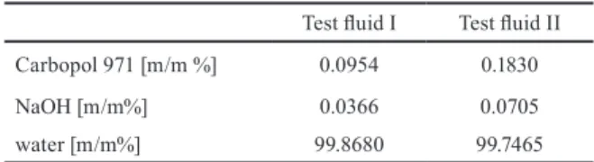
Two different fluids were produced for the examina- tions, Test fluid I and II in the paper. The fluids contained Carbopol 971, NaOH and water. The NaOH was added to set the pH-value to approximately 7. Table 1 shows the exact compositions of the two test fluids.
For determining the rheological parameters of both fluids an Anton PAAR Physica MCR 301 rotational rhe- ometer was used. The investigated shear rate range was 10-1000 1/s, so laminar shear flow conditions occurred during the measurements.
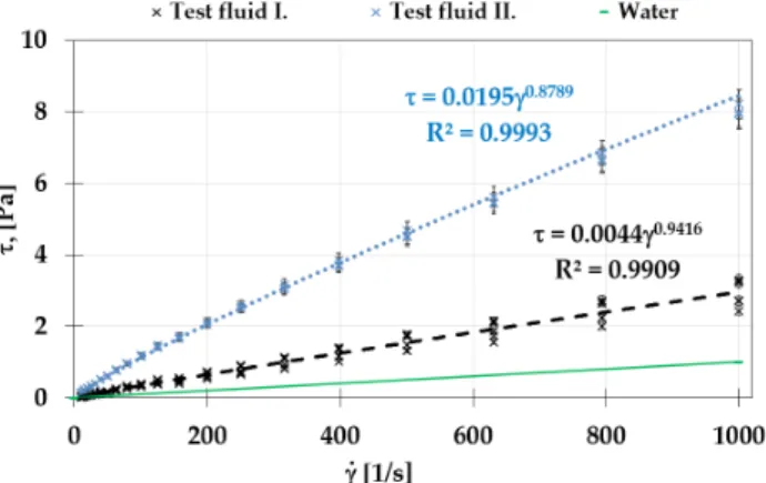
The results of the rheological measurements can be seen in Fig. 1 with a 5 % estimated error bar. The pow- er-law rheology model was chosen to fit to the measured points. The actual values of the curve fit and the coeffi- cients of determination (R2) of the fits can be seen in Table 2.
It is important to note that one order of magnitude differ- ence was between the flow consistency indices of the fluids.
Both of the solutions were found to be pseudoplastic fluid.
2.3 Dimensionless parameters
The Darcy friction factor ( f ) was calculated from the pressure drop in a chosen straight pipe section before the fitting, where the flow was already developed:
f p
L D v
= ∆ ρ 2
2
, (3)
Table 2 Material properties of the two fluids and the coefficients of determination of the fits
Test fluid I Test fluid II
n[-] 0.9416 0.8789
µPL [] 0.0044 0.0195
R2 [-] 0.9909 0.9993
Table 1 The components of the investigated fluids Test fluid I Test fluid II
Carbopol 971 [m/m %] 0.0954 0.1830
NaΟΗ [m/m%] 0.0366 0.0705
water [m/m%] 99.8680 99.7465
in which Δp is the total pressure drop in the pipe section,
ρ is the fluid density (which was approximated with the water density), L is the length of the section, D is the diam- eter of the pipe and v is the average velocity.
The loss coefficient (ξ) was defined as the non-dimen- sional difference in total pressure caused by the fitting:
ξ = ρ∆p v
e
2
2
, (4)
in which Δpe is the total pressure drop caused by the ele- ment. It was calculated between the beginning of the fit- ting and a plane after the elbow in 9D distance. The loss caused by the wall friction was subtracted from it but the forward disturbance of the fitting was taken into consid- eration. It was verified by the authors that beyond 9D the forward impact of the elbow is negligible because there the Δpe changes less than 5 % [28].
Theoretically, the Reynolds number is the ratio of inertial forces to viscous forces; for Newtonian fluids it is given as Re = vDρ/μ. For laminar and fully developed flow, the Darcy friction factor (fD = 64/Re) is defined, which is generally given for fluids independent of their viscosity characteristic [37]. For pipe flow Metzner and Reed [38] introduced a modified Reynolds number valid for power-law fluids, as
Remod = .
+
−
−
v D n
n
n n
n PL
n 2
8 1 3 1
4 ρ µ
(5)
With this modification, the friction factor is f =64 / Remod for laminarflow conditions, see e.g. [28, 37, 39]. This evaluation is useful to compare the results of different power-law fluids with the literature.
In the turbulent zone the Blasius equation for hydrau- lically smooth pipe f =0 316. Re−mod0 25. could be used as an approximation for the friction factor [40].
3 Experiments
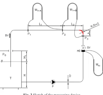
Fig. 2 presents the sketch of the measuring device. The WILO Helix EXCEL 1602-1/16/E/KS variable speed cen- trifugal pump (“P”) delivered the fluid. The flow rate was set by varying the revolution number of the pump. For more sensitive control, a gate valve (“GV”) was used on the discharge-side pipe. The diameter of the pipes (made of steel) was constant DN 40 for the whole system. The investigated 90° bend (marked with red in Fig. 2) had the radius of curvature of R = 80 mm.
The suction pipe of the pump was connected to an open tank (“T”). The “H” fluid level in the tank was kept con- stant at each measurement so that any evaporation did not affect the experimental results. It has been assumed, that this was sufficient to preserve the rheological proper- ties of the fluid between the measurements. The possible time-varying material structure was not taken into con- sideration. The experiments were carried out at constant ambient temperature and air pressure.
An additional butterfly valve (“BV”) was built in to ease the aeration of the manometers (“M1-A” and “M1-B”).
The volume flow rate (Q) was measured with an ori- fice meter (“OM”), which was connected to the “MOM” manometer. This device was calibrated with the non-New- tonian fluid before the measurements. Upstream the ori- fice, a straight pipe section of 25D ensured the uniformity of the streamlines. At the downstream side of the orifice meter, 10D long pipe was found to be sufficient to elimi- nate the disturbances.
Our experiments were divided into two sections:
marked with “A” and “B” assembly.
3.1 Assembly A
The goal of the “A” experiment was to determine the fric- tion factor of the pipe. The mean velocity was calculated from the measured volume flow rate (Q)
v Q
= D4
2π. (6)
The friction factor was calculated with Eq. (3) from the measured pressure drop between the static pressure tap points P1 and P2 with the known L1 length, D diameter and the mean velocity . In these experiments the “M1-A” manometer was used to measure the pressure drop (Δp).
Fig. 1 Measured and fit rheograms of the test fluids.
black dashed line: Test fluid I; blue dotted line: Test fluid II; green solid line: water (as reference)
The P2 point was more than 10D distance at down- stream side of the elbow, so we could assume persistent flow conditions in the measuring region.
3.2 Assembly B
The loss coefficient (ξ) of the elbow with an R/D = 2 rela- tive radius of curvature was determined by the “B” exper- iment. The pressure drop (Δp) was measured by the “M1-B” manometer between the P2 and P3 points. The pressure loss caused by the wall friction in this pipe-section (character- ized with a reference length Lref = 11.25D) was subtracted from this value to get the Δpe pressure loss on the elbow
∆p ∆p f L D v
e= − e ref ρ
2
2, (7)
where fe was the friction factor. For estimation of fe in laminar region the Darcy equation; in turbulent zone the Blasius equation was used. The Δpe and the mean velocity were used in Eq. (4) to specify the measured loss coeffi- cient [41].
3.3 Experimental procedure
Before the experiments, aerations of the manometers were completed and the fluid level of the tank was adjusted to the prescribed value.
The same Reynolds numbers were set for both measure- ment series to obtain comparable results. To achieve this, we took care of the accuracy of the adjustment of the vol- ume flow rate.
The measurements were started at the lowest possible speed of rotation (nrpm = 1000 rpm) with almost completely closed gate valve. After that the gate valve was opened in 6-8 steps at the same constant speed. The additional points were adjusted by increasing the speed of revolution in 300 rpm steps. This resulted further 8 measuring points in the high Reynolds number region.
During a measuring sequence, in every operation point the levels of MOM and the M1-A or M1-B manometers were recorded. The accuracy of the readings was ±1mm.
The whole procedure was repeated with the other fluid as well.
At each measurement point we made an error estimation.
4 Numerical model and simulation setup
The geometry for the CFD simulations was built in Autodesk Inventor Professional 2015 (Student version), and its dimensions were exactly the same as those of the mea- suring device. The model consisted of a 5D long straight pipe before the elbow, the 90° pipe bend and another 10D long pipe section after the fitting. The schematic illustra- tion of the model can be seen in Fig. 3.
The meshing procedure and the simulations were car- ried out in ANSYS CFX®. This software solves the con- tinuity equation, the Reynolds-averaged Navier-Stokes equation (RANS), and the turbulent transport equations (see [29, 41, 42]). Furthermore, the material model describ- ing the rheology gives the relationship between the defor- mation and tension tensors. We used the built-in k-ω SST turbulence model. A detailed description of the program package can be found in [42].
At the upstream boundary uniform velocity profile was prescribed; at downstream average static pressure was imposed as boundary condition. Hydraulically smooth friction wall was defined. Three dimensional structured mesh geometry containing O-grid type elements was used, which consisted of ~160k elements, the maximum and minimum sizes were 6 and 0.25 mm. A numerically finer mesh was applied near the wall for better resolution of the boundary layer.
The grid-independence study, which tested three numerical resolutions containing approximately 80k, 160k and 320k elements, proved the mesh to be sufficient for our task. The difference of the results from the first and third above mentioned model are 1.7 % and 0.4 %, respectively.
Steady state simulations were performed. We used the automatic time-step manager and the convergence criteria of (RMS) for the calculations.
Fig. 2 Sketch of the measuring device
red: 90°pipe bend; P: pump; OM: orifice meter; GV: gate valve; BV:
butterfly valve; M0M, M1-A and M1-B: U tube manometers; P1, P2, P3: pressure measuring places; T: feeding tank.
Additional planes for processing the numerical results were defined at φ = {0°; 22.5°; 45°; 67.5°; 90°} and in the distance of 1D after the bend to visualize the flow patterns (see Fig. 3).
5 Results
5.1 Friction factor
The friction factor of the pipe was used to validate our numerical results. The measured and calculated friction factor of the pipe can be depicted as the function of the modified Reynolds number, see in Figs. 4. and 5.
The analytical friction factors with the known Darcy and Blasius equations were also calculated for the laminar and turbulent regions to compare our results with them.
We obtained numerical and analytical results in the whole investigated modified Reynolds number region (Remod = 100 – 100 000), but the measurements were carried out only in the transition and turbulent zones. The error of the experiments was also estimated and shown on the dia- grams in Figs. 4. and 5. The possible error of the modified Reynolds number was not to taken into account because its relative value was negligible in the turbulent region, where the majority of our points are located.
In case of Test fluid I the relative error of the friction factor calculated from the measured pressure drop was below 10 % in the turbulent zone. The highest relative error (37 %) was detected at the lowest measured velocity.
The measured and the numerical friction factors showed a good correlation. Slightly higher difference between our and the analytical friction factors was detected in the region of Remod = 1500 – 5000. This can be explained by the fact that the transition region may have shifted in the case of this material properties into this region.
We compared the measured and analytical factors as well. The highest difference was 25 % at Remod = 1 549 between the measured and Darcy friction values in the transition zone. At the beginning of the turbulent region a remarkable 15 % difference was between the measured and those calculated with the Blasius equation. Apart from this we found a very good consistency.
At higher Reynolds number (Remod > 10 000) the dif- ference between the numerical and measured results was within the experimental error band, and it was below 5 % between the analytical and the numerical ones.
The friction factors were also calculated in the case of more viscous fluid, Test fluid II, see in Fig.
5. Measurements were performed in the modified Reynolds number range of Remod = 700 – 20 000. The highest value of the relative error of the measured friction factors was estimated to be 51 % at Remod = 722; apart from this the relative error was below 8 %.
Fig. 3 Sketch of the CFD geometry. Additional planes for processing the numerical results were defined at φ = {0°; 22.5°; 45°; 67.5°; 90°}
angles and in the distance of 1D after the bend.
Fig. 4 Experimental (red cross), numerical (blue plus sign) and analytical Darcy (black line) and Blasius (green line) friction factor plotted against the modified Reynolds number in case of Test fluid I
Fig. 5 Experimental (red cross), numerical (blue plus sign) and analytical Darcy (black line) and Blasius (green line) friction factor
against the modified Reynolds number in case of Test fluid II
The high relative errors at the lowest measured points in Figs. 4 and 5 can be clarified, because in those points the exact value of the manometer readings and the absolute error were comparable. To eliminate these inaccuracies in the future, a more accurate pressure gauge would be needed in the range of low pressure differences.
In the laminar region the numerical, analytical and experimental values showed a good agreement.
In the transition and turbulent zones, the measured and calculated friction factors agreed as well. At higher than Remod ≈10 000 these results were fit to the analyti- cal Blasius equation. The maximum discrepancy between the measured and calculated factors was 18 %, which was detected in the transition zone.
These results suggest, that our CFD method gave appli- cable and accurate results.
5.2 Loss coefficients
Fig. 6 shows the loss coefficient of the 90° bend as the function of the modified Reynolds number. CFD calcula- tions were performed in a wide Reynolds number range; in contrast, the measured range was limited. With Test fluid I we were able to measure satisfying results only in the tur- bulent zone; while with Test fluid II measurements in the transition zone were feasible with our equipment.
Besides our measured and numerical coefficients, we also depicted the experimental results of Miller [12], who investigated experimentally an elbow with the same geometry in a wide range of the Reynolds number using water. Our measured and calculated coefficients were in almost the whole region above those from Miller’s work by a max. factor of 2.
In the turbulent region, which is interesting in indus- trial applications, our experimental and numerical results agreed very well. This confirms the usefulness of the modified Reynolds number again.
5.3 Velocity profiles
From an industrial point of view, the pressure drop of a fitting at a given volume flow rate is the most important data. The pressure drop- mean velocity function shows, that in case of Test fluid II higher pressure losses on the elbow appeared in the whole Remod region, see in Fig. 7.
The diagram in Fig. 7 presents also the results of the water as reference.
Conveying different fluids can cause significantly differ- ent flow conditions. Based on the literature, the modifica- tion of the Reynolds number eliminated these differences;
the same flow pattern was created at the same modified Reynolds numbers. To ensure this statement the flow pat- tern at the value of Remod ≈ 20 500 and at the mean veloc- ity of v ≈ 1m/s were investigated with both of the fluids.
The exact conditions of the two analyzed flow circumstances are given in Table 3; all four examples were from the turbu- lent region. (The loss coefficients values for these flows are marked with yellow and green boxes in Fig. 6.) The normal- ized axial velocity profiles along the elbow in the symmetry plane at the defined places can be seen in Fig. 8.
The upper diagram in Fig. 8 shows that the velocity pat- tern at Remod ≈ 20 500 was similar for the two fluids: the aver- age relative difference between the two normalized profiles was below 1 %. In contrast, at mean velocity of v = 1 m/s significant differences between the velocity profiles were observed. The average relative difference was 10 %; the highest was 65 % between the normalized velocity values.
In the final part of the survey the velocity magnitude in the bend was investigated, see Fig. 9. Even though the magnitude of the velocity was more than 2.5 times higher
Fig. 7 Experimental and numerical (CFD) pressure drop of the elbow as the function of the mean velocity for Test fluid I, II and water (as
reference)
Fig. 6 Experimental and numerical (CFD) loss coefficient of the elbow plotted against the modified Reynolds number for Test fluid I and II
for Test fluid II at Remod ≈ 20 500, there was no qualita- tive difference between the two flows in the symmetry plane. In contrast, at v =1 m/s there was a visible differ- ence between the patterns.
We originated the Dean numbers from the modified Reynolds number De=Remod(D/2R)0.5. At the investigated situations De numbers were higher than 2 000. It is known that fully turbulent flow forms after De > 400, so turbu- lent flow were expected to occur in the bends.
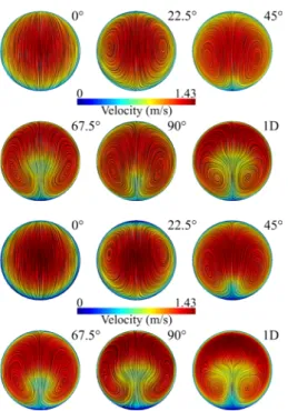
As in the case of the normalized velocity profiles, secondary contour plots showed the same results at Remod ≈ 20 500. Although the mean velocity with Test fluid II was significantly higher than that with Test fluid I, the contour plots did not differ in the two states, see in Fig. 10.
The focus points of the secondary vortices and the quality of the velocity pattern almost completely agreed.
Fig. 11 shows that neither the swirls formed nor the velocity pattern matched in the two cases of mean veloc- ity v = 1 m/s.
6 Conclusions
The main purpose of the current study was to compare the measured and calculated losses of a 90° pipe bend in case of two power-law fluids with significantly different rheol- ogy. The second aim was to investigate the flow pattern in the fitting and to test the generalization of the modified Reynolds number.
Table 3 The conditions of the investigated flows Test fluid I Test fluid II 1.
Remod [-] 20 517 20 544
v [m/s] 1.633 4.531
ξ [-] 0.326 0.290
2.
Remod [-] 12 947 4 019
v [m/s] 1.057 1.057
ξ [-] 0.390 0.446
Fig. 8 Normalized axial velocity profiles along the elbow in the symmetry plane at Remod= 20 500 (top) and at v = 1 m/s (bottom) mean
velocity for both fluids.
black: Test fluid I; blue dashed: Test fluid II
Fig. 9 Velocity magnitude in the symmetry plane of the elbow at Remod= 20 500 (top) and at v = 1 m/s (bottom) mean velocity
for Test fluid I (left) and Test fluid II (right)
Fig. 10 Secondary flow contour plots and velocity along the elbow at the surfaces defined in Fig. 3 at Remod = 20 500;
top: Test fluid I; bottom: Test fluid II
The investigation of the friction factor in a straight pipe section suggested, that the CFD simulations and the applied turbulence model (k-ω SST) is perfectly suited for our tasks. The calculated friction factors showed reason- able agreement with the experiments and analytical values.
Based on the analysis of the velocity vectors and sec- ondary flow structures, the modification of the Reynolds number is strongly recommended.
The third major finding was that the loss coefficient as the function of the modified Reynolds number were determined, and the results can be useful in the sizing of hydrodynamic systems, if the fluid has power-law rheological properties.
Acknowledgement
The research reported in this paper was supported by the Higher Education Excellence Program of the Ministry of Human Capacities in the frame of Water Science &
Disaster Prevention research area of Budapest University of Technology and Economics (BME FIKP-VÍZ). This paper was also supported by the Peter Csizmadia's János Bolyai Research Scholarship of the Hungarian Academy of Sciences.
Nomenclature
D inner diameter of the pipe and the bend [m]
De Dean number [-]
f friction factor [-]
fD Darcy friction factor [-]
fe estimated friction factor of the element [-]
L length of a pipe section [m]
Lref reference length of the elbow [m]
n flow behaviour index [-]
nrpm speed of rotation [rpm]
r radial coordinate [m]
R radius of the curvature [m]
R2 coefficients of determination [-]
Re Reynolds number [-]
Remod modified Reynolds number [-]
Q volume flow rate [m3/s]
v , v mean flow velocity [m/s]
γ shear rate [1/s]
Δp total pressure drop in the pipe section [Pa]
Δpe total pressure drop caused by the element [Pa]
η dynamic viscosity [Pa s]
µPL flow consistency [Pa sn] ρ fluid density [kg/m3] τ shear stress [Pa]
ξ loss coefficient [-]
φ angular position of the defined planes [°]
Fig. 11 Secondary flow contour plots and velocity along the elbow at the surfaces defined in Fig. 3 at v = 1 m/s mean velocity;
top: Test fluid I; bottom: Test fluid II
References
[1] Fozer, D., Sziraky, F. Z., Racz, L., Nagy, T., Tarjani, A. J., Toth, A. J., Haaz, E., Benko, T., Mizsey, P. "Life cycle, PESTLE and Multi-Criteria Decision Analysis of CCS process alternatives", Journal of Cleaner Production, 147, pp. 75–85, 2017.
https://doi.org/10.1016/j.jclepro.2017.01.056
[2] Haaz, E., Fozer, D., Nagy, T., Valentinyi, N., Andre, A., Matyasi, J., Balla, J., Mizsey, P., Toth, A. J. "Vacuum evaporation and reverse osmosis treatment of process wastewaters containing surfactant material: COD reduction and water reuse", Clean Technologies and Environmental Policy, 21(4), pp. 861–870, 2019.
https://doi.org/10.1007/s10098-019-01673-5
[3] Nagy, J., Kaljunen, J., Toth, A. J. "Nitrogen recovery from waste- water and human urine with hydrophobic gas separation mem- brane: experiments and modelling", Chemical Papers, 73(8), pp. 1903–1915, 2019.
https://doi.org/10.1007/s11696-019-00740-x
[4] Szabados, E., Jobbágy, A., Tóth, A. J., Mizsey, P., Tardy, G., Pulgarin, C., Giannakis, S., Takács, E., Wojnárovits, L., Makó, M., Trócsányi, Z., Tungler, A. "Complex Treatment for the Disposal and Utilization of Process Wastewaters of the Pharmaceutical Industry", Periodica Polytechnica Chemical Engineering, 62(1), pp. 76–90, 2018.
https://doi.org/10.3311/PPch.10543
[5] Gu, J., Xu, G., Liu, Y. "An integrated AMBBR and IFAS-SBR pro- cess for municipal wastewater treatment towards enhanced energy recovery, reduced energy consumption and sludge production", Water Research, 110, pp. 262–269, 2017.
https://doi.org/10.1016/j.watres.2016.12.031
[6] Fan, J., Eves, J., Thompson, H. M., Toropov, V. V., Kapur, N., Copley, D., Mincher, A. "Computational fluid dynamic analysis and design optimization of jet pumps", Computers and Fluids, 46(1), pp. 212–217, 2011.
https://doi.org/10.1016/j.compfluid.2010.10.024
[7] Zhang, Z., Zeng, Y., Kusiak, A. "Minimizing pump energy in a wastewater processing plant", Energy, 47(1), pp. 505–514, 2012.
https://doi.org/10.1016/j.energy.2012.08.048
[8] Benedict, R. P., Carlucci, N. A. "Handbook of Specific Losses in Flow Systems", Plenum Press Data Division, Springer, New York, NY, USA, 1966.
https://doi.org/10.1007/978-1-4684-6063-6
[9] Zierep, J., Bühler, K. "Vertiefende Übungsaufgaben" (Strengthening Practices), In: Zierep, J., Bühler, K. Grundzüge der Strömungslehre, Springer, Offenburg, Germany, pp. 161–185, 2010. (in German) https://doi.org/10.1007/978-3-8348-9756-5_5
[10] Idelchik, I. "Handbook of hydraulic resistance", Begell House Inc., New York, NY, USA, 2003.
[11] Mays, L. W. "Water Distribution Systems Handbook", McGraw- Hill and American Water Works Association, Scottsdale, AZ, USA, 2000.
[12] Miller, D. S. "Internal flow systems", BHRA Fluid Engineering Serie, Carnfield, UK, 1978.
[13] Unluturk, S., Atılgan, M. R., Baysal, A. H., Tarı, C. "Use of UV-C radiation as a non-thermal process for liquid egg products (LEP)", Journal of Food Engineering, 85(4), pp. 561–568, 2008.
https://doi.org/10.1016/j.jfoodeng.2007.08.017
[14] Polizelli, M. A., Menegalli, F. C., Telis, V. R. N., Telis-Romero, J.
"Friction losses in valves and fittings for power-law fluids", Brazilian Journal of Chemical Engineering, 20(4), pp. 455–463, 2003.
http://doi.org/10.1590/S0104-66322003000400012
[15] Nagy-György, P., Hős, C. "A Graphical Technique for Solving the Couette-Poiseuille Problem for Generalized Newtonian Fluids", Periodica Polytechnica Chemical Engineering, 63(1), pp. 200–209, 2019.
https://doi.org/10.3311/PPch.11817
[16] Csizmadia, P. "Sűrűzagy keverőben lezajló áramlási folya- matok kísérleti és numerikus vizsgálata" (Experimental and numerical investigation of the flow field inside a dense slurry mixer), PhD Thesis, Budapest University of Technology and Economics, 2016. (in Hugarian)
[17] Csizmadia, P., Hős, C. "LDV measurements of Newtonian and non-Newtonian open-surface swirling flow in a hydrodynamic mixer", Periodica Polytechnica Mechanical Engineering, 57(2), pp. 29–35, 2013.
https://doi.org/10.3311/PPme.7045
[18] Cabral, R. A. F., Telis, V. R. F., Park, K. J., Telis-Romero, J.
"Friction losses in valves and fittings for liquid food products", Food and Bioproducts Processing, 89(4), pp. 375–382, 2011.
https://doi.org/10.1016/j.fbp.2010.08.002
[19] Liu, M., Duan, Y. F. "Resistance properties of coal-water slurry flowing through local piping fittings", Experimental Thermal and Fluid Science, 33(5), pp. 828–837, 2009.
https://doi.org/10.1016/j.expthermflusci.2009.02.011
[20] Etemad, S. G. "Turbulent flow friction loss coefficients of fit- tings for purely viscous non-newtonian fluids", International Communications in Heat Mass Transfer, 31(5), pp. 763–771, 2004.
https://doi.org/10.1016/S0735-1933(04)00063-6
[21] Leal, A. B., Calçada, L. A., Scheid, C. "Non-Newtonian fluid flow in ducts: Friction factor and loss coefficients", In: 4th MERCOSUR Congress on Process Systems Engineering : 2nd MERCOSUR Congress on Chemical Engineering : Proceedings of ENPROMER 2005, Rio de Janeiro, Brazil, pp. 1–10, 2005
[22] Pinho, F. T., Whitelaw, J. H. "Flow of non-newtonian fluids in a pipe", Journal of Non-Newtonian Fluid Mechanics,34(2), pp. 129–144, 1990.
https://doi.org/10.1016/0377-0257(90)80015-R
[23] Bandyopadhyay, T. K., Kumar Das, T. "Non-Newtonian pseu- doplastic liquid flow through small diameter piping compo- nents", Journal of Petroleum Science and Engineering, 55(1–2), pp. 156–166, 2007.
https://doi.org/10.1016/j.petrol.2006.04.006
[24] Verba, A., Embaby, M. H., Angyal, I. "Experimental Measurements on Non-Newtonian and Drag Reduction Flows in Pipes", Periodica Polytechnica Chemical Engineering, 27(1), pp. 57–69, 1983.
[25] Khandelwal, V., Dhiman, A., Baranyi, L. "Laminar flow of non-Newtonian shear-thinning fluids in a T-channel", Computer and Fluids, 108, pp. 79–91, 2015.
https://doi.org/10.1016/j.compfluid.2014.11.030
[26] Kfuri, S. L. D., Silva, J. Q., Soares, E. J., Thompson, R. L. "Friction losses for power-law and viscoplastic materials in an entrance of a tube and an abrupt contraction", Journal of Petroleum Science and Engineering, 76(3–4), pp. 224–235, 2011.
https://doi.org/10.1016/j.petrol.2011.01.002
[27] Ternik, P., Marn, J., Žunič, Z. "Non-Newtonian fluid flow through a planar symmetric expansion: Shear-thickening fluids", Journal of Non-Newtonian Fluid Mechanics, 135(2–3), pp. 136–148, 2006.
https://doi.org/10.1016/j.jnnfm.2006.01.003
[28] Csizmadia, P., Till, S. "The Effect of Rheology Model of an Activated Sludge on to the Predicted Losses by an Elbow", Periodica Polytechnica Mechanical Engineering, 62(4), pp. 305–311, 2018.
https://doi.org/10.3311/PPme.12348
[29] Tezel, G. B., Yapici, K., Uludag, Y. "Numerical and Experimental Investigation of Newtonian Flow Around a Confined Square Cylinder", Periodica Polytechnica Chemical Engineering, 63(1), pp. 190–199, 2019.
https://doi.org/10.3311/PPch.12377
[30] Tezel, G. B., Yapici, K., Uludag, Y. "Flow Characterization of Viscoelastic Fluids around Square Obstacle", Periodica Polytechnica Chemical Engineering, 63(1), pp. 246–257, 2019.
https://doi.org/10.3311/PPch.12426
[31] Dean, W. R. "Note on the Motion of Fluid in a Curved Pipe", Philosophical Magazine Series 7, 4(20), pp. 208–223, 1927.
[32] Marn, J., Ternik, P. "Laminar flow of a shear-thickening fluid in a 90° pipe bend", Fluid Dynamics Research, 38(5), pp. 295–312, 2006.
https://doi.org/10.1016/j.fluiddyn.2006.01.003
[33] Röhrig, R., Jakirlić, S., Tropea, C. "Comparative computa- tional study of turbulent flow in a 90° pipe elbow", International Journal of Heat Fluid Flow, 55, pp. 120–131, 2015.
https://doi.org/10.1016/j.ijheatfluidflow.2015.07.011
[34] Kalpakli, A. "Experimental study of turbulent flows through pipe bends", Royal Institute of Technology KTH Mechanics, Stockholm, Sweden, 2012.
[35] Lajos, T. "Az áramlástan alapjai" (The basics of the flow), Eötvös Kiadó, Budapest, 2008. (in Hungarian)
[36] Litvai, E. "Válogatott fejezetek az áramlástan köréből - Nem- Newtoni folyadékok mechanikája" (Selected chapters of the fluid dynamics - Mechanics of non-Newtonian fluids), Tankönyvkiadó, Budapest, Hungary, 1965. (in Hungarian)
[37] Madlener, K., Frey, B., Ciezki, H. K. "Generalized reynolds num- ber for non-Newtonian fluids", Progress in Propulsion Physics, 1, pp. 237–250, 2009.
https://doi.org/10.1051/eucass/200901237
[38] Metzner, A. B., Reed, J. C. "Flow of non-newtonian fluids-correla- tion of the laminar , transition , and turbulent-flow regions", AlChE Journal, 1(4), pp. 434–440, 1955.
https://doi.org/10.1002/aic.690010409
[39] Eshtiaghi, N., Markis, F., Yap, S. D., Baudez, J. C., Slatter P.,
"Rheological characterisation of municipal sludge: A review", Water Reserach, 47(15), pp. 5493–5510, 2013.
https://doi.org/10.1016/j.watres.2013.07.001
[40] Turian, R. M., Ma, T. W., Hsu, F. L. G., Sung, D. J. "Flow of Concentrated Non-Newtonian Slurries: 1. Friction Losses in Laminar, Turbulent and Transition Flow Through Straight Pipe", International Journal of Multiphase Flow, 24(2), pp. 225–242, 1998.
https://doi.org/10.1016/S0301-9322(97)00038-4
[41] Csizmadia, P., Hős, C. "CFD-based estimation and experiments on the loss coefficient for Bingham and power-law fluids through dif- fusers and elbows", Computers and Fluids, 99, pp. 116–123, 2014.
https://doi.org/10.1016/j.compfluid.2014.04.004
[42] ANSYS "ANSYS CFX-solver theory guide", ANSYS CFX Release, 15317, pp. 724–746, 2009.


![Table 3 The conditions of the investigated flows Test fluid I Test fluid II 1. Re mod [-] 20 517 20 544 v [m/s] 1.633 4.531 ξ [-] 0.326 0.290 2](https://thumb-eu.123doks.com/thumbv2/9dokorg/775104.35056/7.892.515.776.729.1094/table-conditions-investigated-flows-test-fluid-test-fluid.webp)