Biometry

(1)

Biometry

All rights reserved. No part of this work may be reproduced, used or transmitted in any form or by any means – graphic, electronic or mechanical, including photocopying, recording, or information storage and retrieval systems – without the written permission of the author.

(2)

Biometry

Introduction to Statistical Inference

Author:

Judit Poór, associate professor

Reviewers:

Zsuzsanna Bacsi, associate professor László Menyhárt, associate professor

University of Pannonia

Georgikon Faculty

Szent István University

ISBN 978-615-6338-01-3

The textbook was published within the framework of the project EFOP-3.4.3-16-2016- 00009

’Improving the quality and accessibility of higher education at University of Pannonia.’

Keszthely, 2021.

(3)

3

PREFACE

This textbook was written for BSc students, who having completed a course in descriptive statistics, are going to learn the elements of statistical inference. It is also useful for MSc students with no preliminary knowledge of the basic concepts and methods of statistical inference. In a former textbook ‘Descriptive Statistics’ the methods were discussed that are suitable for describing data. In the present textbook some of the methods will be discussed that are suitable to determine the probability that a conclusion drawn from sample data is true.

The textbook presents the application of the methods on data drawn from the agricultural research in Georgikon Faculty reflecting the diversity of research in the Faculty. Many examples compare Hungarian varieties to international ones, including research data from the Department of Animal Sciences, the Department of Corporate Economics and Rural Development, the Department of Horticulture and the Institute of Plant Protection. The author thanks the colleagues of those departments for providing their data for this textbook.

The step-by-step analysis is the best way to analyze biological data. The first steps are in connection with the planning which focuses on the relevant research question:

I.1. Specify the research question.

I.2. Identify the individuals or object of interest.

I.3. Consider whether to use the entire population or a representative sample. In case of sampling, decide on a viable sampling method and do a power analysis if possible, to determine the proper sample size for the experiment.

I.4. Determine the variables relevant to the question, determine the types (e.g. measurement) of variables.

I.5. Remember that there are other variables (called confounding variables), that are not included in the statistical analysis, and plan an experiment that controls or randomizes these confounding variables.

After that the statistical analysis may be broken down into the following steps:

II.1. Do the experiment, collect the data.

II.2. Decide the appropriate descriptive and inferential statistics methods. Put the question to be answered in the form of a statistical null and alternative hypothesis and choose the best statistical test to use.

II.3. Apply appropriate descriptive and inferential statistics methods. Do not forget the assumptions of the chosen statistical analysis. If data fail to meet the assumptions, choose a more appropriate method.

II.4. Interpret the results using graphs or tables, and make decisions.

II.5. Note any important information and concerns that might be important about data collection, or data analysis and list any recommendations for future studies.

The textbook is structured into four chapter. The first chapter explains the basic concepts of probability theory, while the second chapter presents the sampling distributions in statistics.

Statistical inference is a process of drawing conclusions at a certain level of probability. As statistical inference can be divided into two main areas, the third chapter discusses the estimation, while the fourth chapter presents the most basic types of hypothesis testing.

(6)

6

1. INTRODUCTION INTO PROBABILITY DISTRIBUTIONS

Statistical information is used to help decision making. If the population is not actually observed because of constraints on time, money, or effort, the information is considered unknown.

Statistical inference is applied to make statements concerning the unknown information based on sample data, as a generalization from a sample to a population, because a decision based on limited information is always better than a decision without any information. Statistical inference involves drawing a conclusion about a population on the basis of available, sample- based (viz. partial and therefore incomplete) information, so with a certain amount of uncertainty.

Suppose that the likelihood for successful fertilization is examined, or the chance that the newborn calf will be female. The answer to the latter question can be: the gender ratio is 50:50%, but in case of artificial insemination with sexed sperm the gender ratio can reach to 90:10% by high fertility. When probability is used in a question or a statement, a number between 0 and 1 (i.e. from 0% to 100 %) is being used to indicate the likelihood of an event.

The word ‘chance’, ‘predictability’, ‘probability’ is used to indicate the likelihood that some event will happen. These concepts are formalized by the branch of mathematics called probability theory. This chapter will introduce probability concepts. Probability is important in drawing inferences about a population, because statistics deals with drawing inferences applying the rules of mathematical probability. Getting to know the concept of probability leads to the concept of distributions, that is essential in Biometry. Probability theory started to develop on a combinatorial basis. Although mastery of this chapter is not essential to the application of the statistical procedures presented later, occasionally reference will be made to it in the later discussed chapters.

1.1. Events and Sample Space

In statistics an experiment is defined as a process that produces some data. When an experiment is performed the occurrence of a specific event may be interesting. Hooda (2013) emphasizes the difference between the term trial and experiment. Any act performed under given specified – in a formal scientific research inquiry carefully and objectively defined – conditions, may be termed as a trial. The trial is conducted once, twice or any number of times under the same specified conditions, it is called a single-trial experiment, or an experiment with two trials, or any number of trials. Later the experiment will be usually single-trial one, therefore the two terms are used as synonyms.

An experiment generates certain outcomes. The outcome of a random experiment will depend on chance, and cannot be predicted with certainty. The set of all possible outcomes of an experiment is called the sample space (represented by the symbol S), a single outcome is called an element, elementary event or sample point of the sample space. All outcomes of an experiment are known as elementary events (represented by the symbol e). The elements can be listed, when sample spaces are finite: S = {e1, e2, … en}

Suppose a phenomenon can happen in k different ways, but in only one of those ways at a time.

Each possible outcome is referred to as an event.

(7)

7

If a random experiment has a sequence of two steps, that is something can happen k1 different ways and something else can happen k2 different ways, then the number of possible ways for both things to occur is k1 · k2. The counting rule can be extended to determine the number of ways for all n things to occur together (i thing can occur in any one of ki ways): k1 · k2 · k3 ·…·

kn (Zar, 2010).

A sample space can also be described in general terms, for example:

S = {all cows of species y | y is a species}

where the vertical bar ‘|’ is read as ‘such that’ or ‘given’.

An event (represented by the symbol E) can be defined as a subset of the sample space E = {ei, ej, …ek}. Events are usually represented by capital letters. For example, A is the event that one of the newborn calves is female: A = {F-M, M-F}; B is that both of the newborn calves have the ‘same’ sex: B = {M-M, F-F}; and C is that at least one of the newborn calves is female C = {M-F, F-M, F-F}.

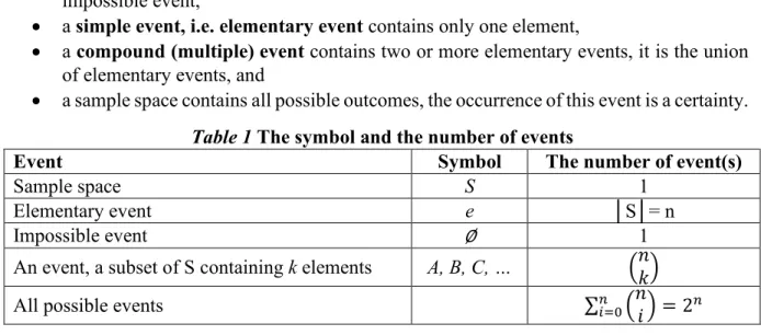
Four types of events can be distinguished (the symbols and the number of events are summarized in Table 1, see the next chapter for the number of events):

 a null or empty space (∅) contains no element of the sample space, such an event is an impossible event,

 a simple event, i.e. elementary event contains only one element,

 a compound (multiple) event contains two or more elementary events, it is the union of elementary events, and

 a sample space contains all possible outcomes, the occurrence of this event is a certainty.

Table 1 The symbol and the number of events

Event Symbol The number of event(s)

Sample space S 1

Elementary event e │S│= n

Impossible event ∅ ¹

An event, a subset of S containing k elements A, B, C, …

All possible events ∑ = 2

EXAMPLE 1.1.1

Some examples of sample spaces are: A cow fertilized is pregnant: S = {Yes, No}

The newborn calf is bull (male – M) or heifer (female – F): S = {M, F}

Age of cow at first calving (months): S = {24, 25, 26, 27, 28, 29, 30, 31}

The number of calves a cow has: S = {0, 1, 2, 3, 4, 5}

The number of calves a cow has in a lifetime: {0, 1, 2, 3, 4, …, 39}

EXAMPLE 1.1.2

Suppose that two cows are calving, a black one and a brown one. There are two possible outcomes for the sex of the newborn calf of the black cow (male or female) and two possible outcomes for the sex of the newborn calf of the brown cow. Therefore, k1 = 2 and k2 = 2 and there are k1 · k2 = 2 · 2 = 4 possible outcomes of the sex of newborn calves:

S = {M-M, F-M, M-F, F-F}.

(8)

8

The complement of an event A is the event (denoted by Ā and read as A bar or A^c) in the sample space containing all the outcomes that are not included in event A. The union of two events A and B is the event (denoted by A∪ B) that contains all the outcomes included either in one or the other of the events A and B, or in both of them. The intersection of two events A and B is the event (denoted by A∩B) that contains all the outcomes common to both A and B. Events A and B are mutually exclusive, if they have no common elements (A∩B = ∅). Any event A and its complement, Ā, are mutually exclusive (disjoint). If all of the elements in event A are also elements of event B, event A is said to be a subset of event B (denoted by A⊂B).

In the context of the sample space of an experiment it should be understood that it is being treated as a population, and a set of outcomes selected from the sample space is being treated as a sample (Hooda, 2013). The concept of these terms is essential to understand the concept of probability. The number of elements in a sample space, and in various events, are often counted to calculate the chance of the events occurring. To determine the number of possible outcomes the multiplication rule, permutations and combinations can be applied.

1.2. Counting Techniques

A permutation is an arrangement of the elements of a set in a specific order. A permutation is one of all possible ways to arrange n distinct objects in an order. If n linear positions are to be filled with n objects, there are n possible ways to fill the first position (k1). The second position can be filled in (n – 1) ways (k2)after the first element is placed in the first position, the third in any one of (n – 2) ways (k3), and so on until the last position, which may be filled in only one possible way (kn). The number of permutations of n distinct objects is

Pn = n ∙ (n-1) ∙ (n-2) ∙ … ∙ 3 ∙ 2 ∙ 1 = n!

(it is read as ‘n factorial’), that is the product of all positive integers from 1 to n by the method of counting rule (by special definition 0! = 1).

If elements are arranged on a circle, there is no starting point as on a line, therefore the number of permutations is !/ . If the orientation of the circle is not specified that is clockwise and counter clockwise patterns are not treated as different, then the number of permutations of n elements is

!

2 = − 1 ! 2 EXAMPLE 1.2.1

A yellow (Y), a red (R), a white (W) and an orange (O) rose are arranged linearly along a fence.

There are 4! = 24 ways to align these four roses:

Y R W O Y R O W Y W R O Y W O R Y O R W Y O W R

R Y W O R Y O W R W Y O R W O Y R O Y W R O W Y

W Y R O W Y O R W R Y O W R O Y W O Y R W O R Y

O Y R W O Y W R O R Y W O R W Y O W Y R O W R Y

(9)

9

If there is no assumed orientation of the observer, these two mirror-image observations can be considered as the same. When we have n elements grouped into k categories, each of which contains ni identical elements (i= 1,…k, and n1 + n2 + … + nk = n) then the number of different permutations is

P ^{, ,…,} = !

∏ !

If n distinct elements are arranged to k (k ≤ n) positions, the number of possible linear permutations of taking k elements from n at a time (denoted by Pnk) is:

P = !

− ! EXAMPLE 1.2.2

A black (B), a grey (G) and a dun (D) horse running in a circle could be arranged in two different ways:

B G D

B

D G P =3!

3 = 2

EXAMPLE 1.2.3

There are five fruit trees, of which three are apple trees (A), and two are pear trees (P). How many different linear sequences of trees are possible?

A A A P P A A P A P A A P P A A P A A P A P A P A

P = 5!

3! · 2! = 10 P A A A P P A A P A P A P A A A P P A A P P A A A

EXAMPLE 1.2.4

Three different varieties of apple trees are bought from an orchard selling fruit trees. The three different varieties can be selected from among Idared (I), Jonagold (J), Mutsu (M), Gloster (G) and Starking (S) apple trees and are planted in order.

There are 5! = 120 ways of placing the 5 varieties in five positions on a line, but there are considerably fewer ways to arrange only three different varieties at a time: P = ^! _!= 60

I J M I J G I J S I M G I M S I G S J M G J M S J G S M G S I M J I G J I S J I G M I S M I S G J G M J S M J S G M S G J M I J G I J S I M G I M S I G S I M G J M S J G S J G S M J I M J I G J I S M I G M I S G I S M J G M J S G J S G M S M I J G I J S I J G I M S I M S I G G J M S J M S J G S M G M J I G J I S J I G M I S M I S G I G M J S M J S G J S G M

(10)

10

There are only !/[ − ! ] ways if the arrangement are circular. The number of possible orders of planting the apple trees in a circle is 60/3=20 (in EXAMPLE 1.2.4 each column contains two circular orders, the ones in italics being in the same circular order, and the rest are also of the same order).

When each trial of the experiment has an equal number of possible outcomes, the total number of outcomes is Pnk,r = n^k, where k is the number of trials and n is the number of outcomes in each trial.

A combination is a selection of a subset from a set without considering the sequence of elements within the subset. In this case only the elements of the subset are important, not their arrangement. The number of combinations of k elements taken from a set of n elements (denoted by Cnk) is

C = ^!_{! !}= (read as ‘n choose k’).

These numbers are called binomial coefficients. The properties of the binomial coefficients are:

0 = = 1 = − = − 1

− 1 + − 1

= 2 − = +

Combination with replacement is defined by the following formula:

C ^, = + − 1

In this case the chosen k elements are not necessarily different, i.e. if six apple trees are to be planted and can be selected from five different varieties, the number of possible ways is

C ^, = 5 + 6 − 16 = 210 EXAMPLE 1.2.5

Assume that the three apple trees bought from the orchard are not necessarily of different varieties. Five different apple tree varieties can be planted into the first place, five varieties can be planted again into the second place, and five varieties into the third place. The number of ways of planting the three apple trees is 5³=125.

EXAMPLE 1.2.6

Referring again to apple trees when the three different varieties are selected from among Idared (I), Jonagold (J), Mutsu (M), Gloster (G) and Starking (S), ignoring the order, the number of ways of selecting 3 out of 5 varieties is 5!/[ 5 − 3 ! 3!] = 10 (since the order of the selected varieties is of no relevance, the choices in each column are the same in EXAMPLE 1.2.4).

(11)

11

The concept of probability has no existence without random sampling. To reach valid conclusions about populations by inference from samples, statistical methods assume random samples. This means that each element of the population has an equal and independent chance of being chosen, that is, the selection of any element has no influence on the selection of any other one. Hunyadi – Vita (2002) emphasize the known probability of the selection of the sample members.

Summarizing the number of the sets of outcomes (sample), the following formulas can be applied (Table 2):

Table 2 The number of the set of outcomes Objective n elements

taken

Replacement

Without With

Arrangement

n at a time Pn = n! ^{, ,…,} = !

∏ !

k at a time

= !

− ! Pnk,r = n^k

Selection = ^, = + − 1

So the random selection of a sample may be done with or without replacement. Sampling with replacement means that the elements are taken one at a time, returning each one to the set before the next one is selected, that is, each element can appear in the sample repeatedly. If each element of a population can be selected only once (and is not replaced), the sampling is done without replacement.

In the following section probability is defined and some rules are introduced. Probability is the language of inferential statistics, and understanding probability is important when interpreting P-values in the statistical tests.

EXAMPLE 1.2.7

If three apple trees would be planted and the three apple trees can be selected in the orchard from five different varieties, then the number of combinations with replacement is

I I I J J J M M M G G G S S S I J M I G S C ^, = 5 + 3 − 13 = 35 I I J J J I M M I G G I S S I I J G J M G

I I M J J M M M J G G J S S J I J S J M S I I G J J G M M G G G M S S M I M G J G S I I S J J S M M S G G S S S G I M G M G S

HOW TO COMPUTE FACTORIALS, PERMUTATIONS AND COMBINATIONS IN EXCEL?

The FACT function is used for computing factorials, the PERMUT function for permutations, and the COMBIN function for combinations.

(12)

12

1.3. Probability

Probabilities are associated with events and are referred to as chances. Probability (P(E), read as ‘P of E’) measures the likelihood of an event (E) with a scale ranging between 0 and 1 often converted to percentages. The value P(E) = 1 (closer to 1) indicates that the event E is certain (very likely) to occur. The value P(E) = 0 (closer to 0) indicates that the event E is certain not (very unlikely) to occur.

A-priori or a-posteriori, empirical and theoretical probabilities can be distinguished. A prior probability is based on knowledge, previous experiences, or is derived by a logical deduction.

A posterior probability is obtained from the prior probability with additional data collected from a planned experiment.

Classical probability, the probability of an event E occurring (P(E)), in general, is defined as

=

where n(E) is the number of ways the event can occur, and N(S) is the total number of outcomes in the sample space.

The empirical probability is calculated based on relative frequency, as a proportion

≈

where f is the number of outcomes not known exactly but observed from a large number (n) of trials. The relative frequency (i.e. the empirical probability) is (very likely) to change from one experiment, and so from one sample, to another for the same E event – from the same population, but the probability can be estimated through repetitive experiments. The relative frequency is approximately equal to the classical probability, i.e. the theoretical value that is expected. The use of the relative frequency approach to assigning probabilities of an event is a common way. According to the law of large numbers, as the number of trials, i.e. the sample size, increases (approaches infinity), the relative frequency approaches the theroretical probability value.

EXAMPLE 1.3.1

What is the chance that the newborn calf will be female?

E might be the event that the newborn calf is female. There are two possible – equally likely – outcomes of the sex of the newborn calf S = {F, M}, therefore the probability of the event E is P(E)

= ½.

If two cows are calving, what is the chance that exactly one of the newborn calves is female (A), both of them have the ‘same’ sex (B), and at least one of the newborn calves is female (C)?

In this case there are 4 possible outcomes of the sex of newborn calves:

S = {M-M, F-M, M-F, F-F}. A = {F-M, M-F}, therefore P(A) = 2/4 = ½,

B = {M-M, F-F}, therefore P(B) = 2/4 = ½, C = {M-F, F-M, F-F}, therefore P(C) = ¾.

(13)

13 The basic probability rules are:

1. The addition rule: If two events A and B are disjoint (with no common intersecting elements) then the probability of the occurrence A or B (union) is the sum of the probabilities of the two events: P(A ∪ B) = P(A) + P(B). The formula can be extended for k disjoint events.

 The probability of an event E = {ei, ej, …, ek} is the sum of the probabilities of the

mutually exclusive elementary events (ei):

P(E) = P(ei) + P(ej) + … + P(ek).

 Since the occurrence of the whole sample space, i.e., all possible outcomes as an event, is a certainty, the sum of the probabilities of all elementary events in a sample space is equal to 1: ∑ = 1.

 As the complement of an event A is the event that A does not occur, A and Ā are mutually exclusive, and A∪ Ā = S, thus P(A ∪ Ā) = P(A) + P(Ā) = P(S) = 1. The probability of a complement is P(Ā) = 1 – P(A).

2. The multiplication law: If two events A and B are independent, that is, the occurrence of event A does not change the probability of the occurrence of event B, and vica versa, then the probability of the occurrence A and B (intersection) is the product of the probabilities of the two events: P(A ∩ B) = P(A) ∙ P(B). The formula can be extended for k mutually independent events.

3. Conditional probability (denoted by P(A│B) read as ‘P(A, given B)’) is the probability of the occurrence of an event (A) with the condition that another event (B) (P(B) ≠ 0) also occurred:

| = ∩

 If the events A and B are independent, then P(A) = P(A│B) = P(A│ ).

 If the events A and B are dependent, then P(A) ≠ P(A│B) and P(A ∩ B) ≠ P(A) ∙ P(B), the change in the probability of event A caused by the occurrence of the other event (B) must be taken into account. So the general multiplication law for any events (Bajpai, 2010) is:

∩ = | ∙ = | ∙ , ℎ | = | ∙

4. The addition rule for two intersecting events A and B can be calculated as:

P(A ∪ B) = P(A) + P(B) – P(A ∩ B).

to avoid the double-counting of the intersection space.

What is the chance that exactly one of the newborn calves is female (A) and both of the newborn calves have the ‘same’ sex (B)?

The two events are disjoint, therefore the probability of the occurrence A and B is 0.

What is the chance that at least one of the newborn calves is female (A) and both of the newborn calves have the ‘same’ sex (B)?

The intersection of the events is {F-F}, the probability of this event is P = ¼.

What is the chance that exactly one of the newborn calves is female (A) or both of the newborn calves have the ‘same’ sex (B)?

The union of the events is the whole sample space, therefore the probability is P = 1.

(14)

14

 If the events A and B are independent, then

P(A ∪ B) = P(A) + P(B) – P(A) · P(B)= P(A) + P(B)∙[1-P(A)].

Because event A occurs either with or without event B, P(A) = P(A∩B) + P(A∩ ). This formula leads to the relation of the conditional and unconditional probabilities.

5. For any events A and B

P(A) = | ∙ + | ∙

The formula can be extended for k disjoint and exhaustive (i.e., when at least one of them must occur) events (B1, B2, …, Bk). The probability of event A is the weighted average of the conditional probabilities of event A given event Bi:

P(A) = ∑ | ∙

 From this relationship the following formula, known as Bayes’ Theorem, is derived:

| = | ∙

= | ∙

∑ | ∙

The value of a categorical or a numeric variable is observed for each sampled element of a population to describe the statistical features of the sample and generalize the sample results to the population. The variables, and the statistics are all random variables.

EXAMPLE 1.3.2

The grape powdery mildew infection risk was 60% in the region of Kőszeg and 80% in the region of Vaskeresztes in 2013. What does it mean? It means, that if a grape is selected in the region of Kőszeg random, the probability of the powdery mildew infection is 60%, that is, if 100 grapes are selected randomly, approximately 60 of 100 is infected, while the same proportion in Vaskeresztes is 80 of 100. Denote A the event, that the grape is infected, and Ā that it is not infected, and B and C the events that the grape is in Kőszeg and Vaskeresztes, respectively. The probability of infection in Kőszeg is P(A│B) = 60% (and of non-infection in Kőszeg is P(Ā│B) = 40%), while the same probabilities in Vaskeresztes are P(A│C) = 80% and P(Ā│C) = 20%.

EXAMPLE 1.3.3

In a region the proportion of resistant grape varieties is 30%. In case of these varieties the powdery mildew infection risk is 5%, while 70% otherwise. What is the chance of the powdery mildew infection of this region? Denote A the event that the grape is infected, Ā that the grape is not infected, and B that the grape is resistant while the event that the grape is not resistant. The probability of infection given a resistant grape variety is P(A│B) = 5%.

Infected (A) Non-infected (Ā) Probability

Resistant (B) P(A│B) = 5% P(Ā│B) = 95% P(B) = 30%

Non-resistant ) P(A│ ) = 70% P(Ā│ ) = 30% P( ) = 70%

To calculate the probability of the powdery mildew infection, the following formula is used:

P(A) = | ∙ + | ∙ = 0.05 ∙ 0.3 + 0.7 ∙ 0.7 = 0.505 = 50.5%

(15)

15

1.4. Probability Distribution

A random variable is a function that assigns numeric values to the outcomes of a random experiment in the sample space. A quantitative variable (denoted by X) measuring the outcome, takes a random numerical value with some probability. Random variables can be:

 discrete: that can take on only particular (i.e., a finite number of) values, and they are the results of a count – often integers (e.g. the number of infected trees, pregnant cows), or

 continuous: that can take on any value in an interval, and they are typically the results of a measurement (the diameter of the tree trunk, the weight of a piece of valuable meat) – real numbers.

A probability distribution is a table, a graph or a formula (a function) that assigns a probability to each value of a random variable. A relative frequency distribution based on an ‘infinitely’

large sample can be considered as a probability distribution. The function f(x) that presents a probability distribution of a discrete variable is called probability mass function. The function that presents a probability distribution of a continuous variable is called probability density function.

A random variable and the associated probability distribution are described by parameters. The expectation or expected value of a variable X is the mean of the random variable, that represents the ‘central-point’ for the entire distribution, the long-term ‘average’value if the experiment is conducted repeatedly. The expected value is not necessarily a value of the sample space:

E(X) = μ_X

The variance of X is the mean square deviation from the mean, the spread, relative to the expected value

Var(X) = σ²_X = E[(X - μ_X)²] = E(X²) – μ_X²

The standard deviation is the square root of the variance, that represents the measure of risk:

the larger the standard deviation, the greater the likelihood that the random variable is different from the expected value. If the Greek letters (μ, σ) are used, the information given about the expected value or the standard deviation is from the entire population.

The cumulative distribution function, denoted by F(x), assigns to each value the sum of probabilities of all values no larger than the considered value (x), and is defined as

F(x) = P(X ≤ x)

The P^th percentile of the distribution is the value such that P% of the data fall at, or below it, and (100-P)% of the data fall at, or above it.

1.4.1. Probability Distribution for a Discrete Random Variable

The probability distribution for a discrete random variable (X) assigns a probability 0 ≤ P(x) ≤ 1 to each distinct value (x) of a discrete random variable. The sum of all possible probability values must equal 1. To present a probability distribution graphically for a discrete random variable a stick plot is the correct type because it does not take on any value between two integers. The values of X are placed along the horizontal axis and the probabilities of the outcomes on the vertical axis.

(16)

16

The expected value of a discrete random variable is the weighted average of all possible values (x) of the variable, where the weights are the probabilities P(x):

μ_X = E(X) = ΣxP(x) The variance of a discrete random variable is:

σ²X = Var(X) = Σ(x-μ_X)²P(x) = Σx²P(x)-μ_X² EXAMPLE 1.4.1

Assume that 5 (n) cows are calving. The probability and the cumulative distribution for the number (x) of the female newborn calves is as follows, where the probability P(x) of the outcomes is:

= = =

x 0 1 2 3 4 5

P(X=x) = = =

F(x) 1

32 6

32 16

32 26

32 31

32 1

The mean and the variance are calculated as:

μ = 0 ∙ 1

32 + 1 ∙ 5

32 + 2 ∙10

32 + 3 ∙10

32 + 4 ∙ 5

32 + 5 ∙ 1 32 =80

32 = 2.5 σ = 0 ∙ 1

32 + 1 ∙ 5

32 + 2 ∙10

32 + 3 ∙10

32 + 4 ∙ 5

32 + 5 ∙ 1

32 − 2.5 = 1.25 σX = 1,25

EXAMPLE 1.4.2

There are five fruit trees, of which three are apple trees (A), two are pear trees (P). Three trees are selected for planting. The probability distribution for the number (x) of planted apple trees is as follows, with the probability P(x) of the outcomes:

= = ∙

x 1 2 3 Σ

P(X=x)

31 2 52 3

= 3 10

32 2 51 3

= 6 10

33 2 50 3

= 1

10 1

The mean and the variance are calculated as:

μ = E X = 1 ∙ + 2 ∙ + 3 ∙ = = 1.8 σ = Var X = 1 ∙ + 2 ∙ + 3 ∙ − 1.8 = 0.36

σX = 0.6

(17)

17

Observations from experiments can be classified and described by a certain probability distribution. It is important to be able to recognize the type of a discrete distribution. The most common probability distributions are the following:

 Uniform distribution: the probability of every outcome is the same (P(X)=1/k, where k is the number of the possible outcomes), the probability function is defined only by one parameter, the number of possible outcomes. The mean and the variance of a discrete uniform variable of consecutive integers between a ≤ b are

= =

If the experiment has two possible outcomes (‘success’ and ‘failure’), the trial and the variable is called binary ~ Bernoulli. This trial is repeated several times (n) under identical conditions.

 Binomial distribution: the probability function for this dichonomous event is defined by two parameters: the number of trials (n), and the probability (p) of the specific preferred outcome (called ‘success’), which is the same for each trial. The trials are independent because binomial probabilities are the result from a sampling with replacement. The probability function for the variable X (0 ≤ x ≤ n) representing the occurrence number of the preferred outcome:

= 1 −

The mean and the variance of a binomial variable are

= =

 Hypergeometric distribution: the probability is not constant, and the trials are not independent because trials are made without replacement. If the population is relatively small, the hypergeometric distribution should be used. If random sample is drawn from a very large population (n < 0.05N), the trials are approximately independent, so the probabilities do not change much and the hypergeometric distribution approaches the binomial one. The probability function for the variable X (0 ≤ x ≤ min(k,n)) representing the number of preferred outcomes (‘successes’) occurring in a sample of n from a set of size N (n < N) with k of them being ‘successes’ that is, the probability of ‘success’ is p = k/N:

EXAMPLE 1.4.3

A biologist is studying a new hybrid plant of which seeds have probability of germinating 0.85 (p).

The biologist plants four (n) seeds. What is the probability that exactly x seeds will germinate, what is the expected number and the standard deviation of germinating seeds?

= 4 0.85 0.15 = 4 ∙ 0.85 = 3.4 = √4 ∙ 0.85 ∙ 0.15 = √0.51=0.7141 The mean and the variance can be also calculated in EXAMPLE 1.4.1, as:

= 5 ∙ 0.5 = 2.5, σ² = 5 ∙ 0.5 ∙ 0.5 = 1.25

(18)

18

=

−−

The mean and the variance of a hypergeometric variable are

= = = 1 − = 1 −

There are distributions in case of which n is not fixed but they give the probability of reaching a particular number of successes (k) from a certain number of trials.

 Negative binomial distribution: gives the probability of reaching the k^th success in the n^th trial

= − 1

− 1 1 − = =

 Geometric distribution: is a special form of the negative binomial distribution, which gives the probability of the first (k = 1) success in the n^th trial.

= 1 − = =

EXAMPLE 1.4.4

In a box there are 2 (k) ill and 10 (N - k) healthy pigs, from which 3 (n) pigs are selected at random.

What is the probability, the expected number and the standard deviation of the number of ill animals in the random selection?

= = 3 = 0.5 = 3 1 − = √0.34

The mean and the variance can be also calculated in EXAMPLE 1.4.2. as μ = 3 = 1.8 σ² = 3 1 − = 0.36

EXAMPLE 1.4.5

In a herd the pregnancy rate of the cows is approximately 40%. Denote n the random variable that represents the number of cows that must be examined to find the first pregnant one. What is the probability distribution of the random variable n, and the expected number of cows to be examined?

= 0.4 0.6 = _. = 2.5

(19)

19

If a distribution of the probability of rare events, occurring infrequently in time or space, is examined, that is, there is a small probability of an occurrence, the distribution is:

 Poisson distribution: the probability distribution of the number of rare events in a fixed time, area, volume or any other quantity that can be subdivided into smaller and smaller intervals, based on long-term experience, with a known average rate over designated intervals (μ = λ), the mean and the variance of the distribution are:

= _! x = 0,1,2,… = =

where e is the base of the natural logarithm, and the only parameter, λ defines the distribution. Binomial distribution can be approximated by a Poisson one if n is large (n > 100) and p is small (np < 10).

EXAMPLE 1.4.6

Approximately 4.0% of untreated Jonathan apples has bitter pit disease. Denote n the random variable that represents the number of apples that must be examined to find the first one with bitter pit. What is the probability distribution of the random variable n, and the expected number of apples that must be examined?

= 0.04 0.96 = _. = 25

EXAMPLE 1.4.7

There are 100 potato plants in a garden, on which 50 Colorado potato beetles randomly land. What is the expected number of beetles per plant and the probability of plants with X = 0,1,2,... beetles?

μ = λ = 0 · 0.6065 + 1 · 0.3033 + ⋯ = = 0.5 beetles/plants Number of beetles X P(X) Estimated numbers of plant

0 0.6065 61

1 0.3033 30

2 0.0758 7

3 0.0126 1

4 0.0016 0

5 0.0002 0

more than 5 0.0000 0

Sum 1 100

(20)

20

1.4.2. Probability Distribution for a Continuous Random Variable

Most variables examined in biology are continuous. In this section distributions of continuous variables are discussed. Assume there is no measurement error and the random variable can take on a continuum of possible values. The probability density function f(x) of the random variable X represents the density for a given value of the variable. Because a continuous variable X can take on infinite possible numbers of values, the probability distribution assigns a probability 0 ≤ P(x) ≤ 1 to each interval of values (between any two limits x1 and x2) of the continuous random variable. The probability of any exact value is always 0 (it is impossible to define the probability of an individual value, therefore P(X ≤ x) = P(X < x)).

P(x1 ≤ X ≤ x2) =

As the variable may potentially have any value, the probability density function can be represented by a continuous curve. The total area under this curve, between the two limits, i.e.

the lowest and the highest outcomes, – that may be an infinite interval ]-∞, ∞[ – must equal 1.

The horizontal axis (abscissa) shows the values of the continuous variable and the frequency or the density is given by the height of the curve (vertical axis/ordinate). Because the probability density function is continuous, the cumulative distribution function is also continuous, and is defined as the anti-derivative or integral of the probability density function f(x) in the interval (-∞, x):

F(x) = P(X ≤ x) = for -∞ < x < ∞

The density function is the first derivative of the cumulative distribution function: f(x) = The cumulative distribution function, the mean and the variance for a continuous random variable have the same meaning as for a discrete distribution.

HOW TO COMPUTE PROBABILITIES FOR A DISCRETE RANDOM VARIABLE IN EXCEL AND IN SPSS?

IN EXCEL: the BINOM.DIST function is used to compute binomial probabilities with the following arguments: the number of successes in trials (x); the number of independent trials (n); and the probability of success on each trial (p).

NEGBINOM.DIST is used to compute negative binomial probabilities with the following arguments: the number of failures (n-k); the threshold number of successes (k, for the geometric distribution k = 1); and the probability of success (p).

The POISSON.DIST function is used to compute the Poisson distribution with the following arguments: the number of events (x); and the expected value (λ).

Each of the above-mentioned functions have a logical parameter value, which is set to FALSE to compute the probability P(x), or TRUE to compute the cumulative probability F(x).

IN SPSS: The values of a new variable x are entered in the data editor. In the menu, choose Transform ►Compute, and in the dialogue box type P_x (F_x) for the target variable and in the function box type Pdf.Binom, Pdf.Hyper, Pdf.Negbin, Pdf.Geom or Pdf.Poisson, respectively, to compute the probability distribution function. Cdf. functions with a similar name are also available to calculate the (cumulative) probabilities in a new column of the data editor.

(21)

21

The expected value of a continuous random variable is the weighted average of all possible values (x) of the variable, where the weights are the probabilities f(x):

μX = E(X) = dx The variance of a continuous random variable is:

σ²X = Var(X) = − = – μx2

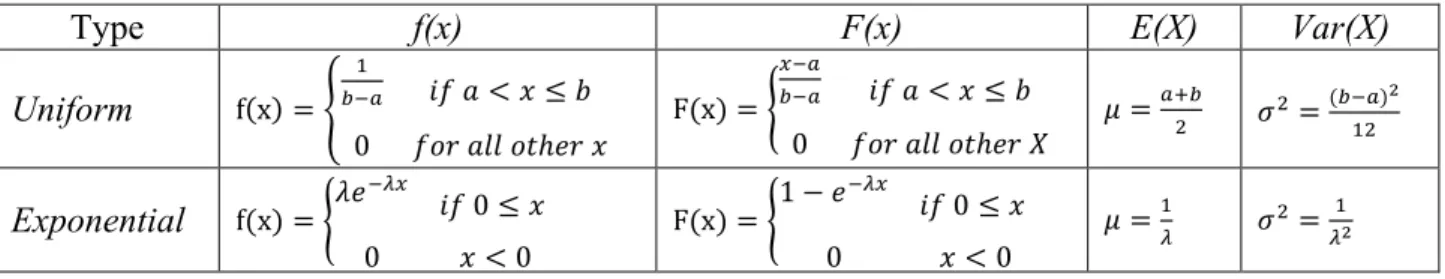
Similarly to discrete probability distributions there are many kinds of continuous distributions to describe the observations gained from experiments. The uniform density is the continuous counterpart to the uniform distribution, and the exponential density is the continuous version to the Poisson distribution.

 Uniform distribution: the meaning is the same as in the case of discrete random variable i.e. the probability of every outcome is equal.

 Exponential distribution: while the probability of the number of rare events (discrete random variable) occurring within a time or space interval is described by the Poisson distribution, the probability of the elapsed times or distances between occurrences of consecutive events is described by the exponential distribution, and both of these distributions are determined by their mean value.

The density, the cumulative distribution function, the mean and the variance of the uniform and the exponential distribution are calculated as in Table 3.

Table 3 The distribution functions and the statistics of uniform and exponential distribution

Type f(x) F(x) E(X) Var(X)

Uniform f x = < ≤

0 ℎ F x = < ≤

0 ℎ = =

Exponential f x = 0 ≤

0 < 0 F x = 1 −

0 ≤

0 < 0 = =

EXAMPLE 1.4.8

Suppose that the length of a 5 m piece of pine slat can be trimmed to any length of between 4.9 m and 5.1 m with equal probabilities. Therefore, the actual slat length is described by a uniform distribution. What is the probability that a piece of slat selected at random is between 4.91 m and 4.95 m?

P 4.91 ≤ x ≤ 4.95 = 1 5.1 − 4.9

,

, =4.95 − 4.91

5.1 − 4.9 =0.04

0.2 = 20%

(22)

22

There are many other continuous distributions (Gamma, Beta, Weibull, Logistic, Cauchy) which are not discussed in this textbook. As the normal probability distribution is the most common and the most important continuous probability distribution in mathematical statistics, therefore it will be explored in more detail.

1.5. The Normal and the Standard Normal Distribution

If the majority of the values tend to be around the mean with progressively fewer observations toward the extreme ends of the range producing ‘tails’ on either side of the distribution, variables and statistics can be characterized by a normal distribution. This distribution is symmetric around its mean (the coefficient of skewness is 0, f(μ) = the maximum of the distribution, and μ = mode = median) and ‘bell-shaped’, although not all bell-shaped curves are normal. The probability function

= 1

√2

which is defined by two parameters the mean and the variance, which specify the position (the balance point = μ) and the extent of spread as well as the height (

√ ) of the curve of the normal distribution. The shorthand expression for this distribution is N(μ,σ²). Any normal random variable X can be transformed (standardized) to standard normal variable as:

= −

Thus X = zσ + μ, that is, the z value shows how many standard deviations a value is above or below the mean value. The mean of the standard normal distribution is always 0 (in standard units), and the variance is always 1; Z~ N(0,1). A positive z value corresponds to a value above the mean in the original distribution, while a value below the mean has a negative z score. The standard score describes the location of the value of the original variable from the mean in standard deviation units.

EXAMPLE 1.4.9

A tractor part can work for 1 000 hours on average without failure (Hunkár, 2011). What is the chance that the tractor will actually work

 for less than 5 000 hours? = 1000 = < 5000 = 1 − = 1 −

 for more than 12 000 hours without failure? > 12000 = 1 − 1 − =

HOW TO COMPUTE PROBABILITIES FOR AN EXPONENTIAL RANDOM VARIABLE IN EXCEL AND IN SPSS?

IN EXCEL: the EXP.DIST function is used to compute exponential probabilities with the following arguments: the value of the function (x); the parameter value (λ); and a logical value which is set to FALSE to compute the probability P(x), or TRUE to compute the cumulative probability F(x).

IN SPSS: The procedure is the same as with discrete distributions with the Pdf.Exp and Cdf.Exp.

(23)

23

The properties of the normal and the standard normal distribution (Figure 1) are:

 The curve is symmetric, the skewness (the measure of the symmetry) is 0, while the mean, median and mode all have the same value, half of the values fall above the mean.

Figure 1 The standard normal distribution and its cumulative distribution function, Z ~ N(0,1)

Source: Rosner (2011)

 The cumulative distribution function of a N(0,1) variable us usually denoted by ϕ(z).

 The kurtosis (the measure of relative peakedness of a probability distribution) is also 0.

 The curve approaches the X-axis asymptotically, that is, the tails of the curve, while moving away from the mean, approach the X-axis, but they never quite reach it.

 Around 68% (slightly over two-thirds) of the area under the curve falls within one standard deviation on each side of the mean, roughly 95% is between μ-2σ and μ+2σ¹.

The probability of a normal random variable between two bounds (x1 and x2) is determined by:

P x¹ ≤ X ≤ x² = P z¹ ≤ Z ≤ z²

i.e., the area under the normal curve, for which the integration should be computed. For convenience the procedure is to transform the bounds into standard z scores first, then look up the probabilities of these standard scores in a z-table. The z-table contains the values of the cumulative probability distribution denoted by ϕ(z) = P(Z < z), the probability of the standard normal variable Z being ‘less than’ a given z-value.

1 By Chebyshev’s Theorem, that the data spread about the mean can be given for all distributions: for a constant k (k > 1) the proportion of values within k standard deviations above or below the mean is at least 1-1/k².

(24)

24

The structure of the z-table (Table A.1 in APPENDICES) is the following: increments of z in tenths in the leftmost column, and increments in hundredths added to these values across the rows. Linear interpolation of the p-values can result in an approximation if a z-value with more than two decimals is required. For example, to find the probability ϕ(0.36) look up the row with 0.30 in the first column of the table, and the column with 0.06 in the first row. The value in the intersection of the chosen row and column, i.e. 0.6406 is the required probability. If we need ϕ(0.365) take the average of ϕ(0.36)=0.6405 and ϕ(0.37)=0.6443, i.e. ϕ(0.365)=0.64245.

The following rules show the way to compute the probabilities:

 P(Z ≥ z): use the rule of complements P(Z ≥ z) = 1 – P(Z < z),

 P(Z ≤ -z): from the symmetry properties P(Z ≤ -z) = P(Z ≥ z),

 P(z1 ≤ Z ≤ z2): the following formula can be used P(Z ≤ z2) – P(Z ≤ z1).

A binomial distribution can be approximated by a normal distribution with (μ = np, σ²=np(1- p)), if np(1-p) ≥ 5 or np ≥ 5 and n(1-p) ≥ 5. A Poisson distribution also can be approximated by a normal distribution with (μ = σ²), if μ ≥ 10.

Why is the normal distribution important?

 Many statistical tests assume, that the data come from a normal distribution.

 The mean and the variance are not dependent on each other for normally distributed data.

 Many natural phenomena are, in fact, more or less normally distributed, that is, the curves illustrating the measures of the phenomena would be close to symmetric around their mean and look like the general bell shape.

EXAMPLE 1.5.1

In a pig farm the average weight of three-month piglets is 35 kg, the weight is normally distributed, with a standard deviation of 6 kg (Hunkár, 2011). Randomly choosing a piglet, compute the chance of its weight being:

less than 32 kg? P(X < 32) = P(Z< = P(Z<-0.5) = P(Z >0.5)=1– P(Z<0.5)=1– 0.3085=0.6915 more than 38 kg? P(X > 38) = 1 – P(X ≤ 38) = 1 – P(Z < = 1 – P(Z < 0.5) = 0.3085

between 36 and 37 kg? P(36 ≤ Z ≤ 37) = P( ≤ Z ≤ ) = P(Z < ) – P(Z < ) = 0.6293 – 0.5675 = 0.0618

EXAMPLE 1.5.2

What is the weight that the heaviest 5% of piglets exceed? If P(Z ≥ z) = 0.05, then P(Z < z) = 0.95. The approximate z score associated with the specific probability can be found from the inverse standard normal distribution. From table A1, using interpolation we get that approximately 5% of piglets are at least 1.645 standard deviations above the mean weight: X0,95 = zσ + μ = 1,645 ∙ 6 + 35 = 44.87 kg, thus the heaviest 5% of piglets are 44.87 kg or heavier, that is P(Z ≥ 1.645) = P(X ≥ 44.87) = 0.95.

(25)

25

 Central Limit Therorem: the distribution of the means of samples taken from even a non-normal distribution can be normally distributed if the sample size is large enough.

When an infinite number of successive random samples of n elements are taken from a population, the sampling distribution of the means of those samples will become approximately normally distributed with mean μ and standard deviation /√ , irrespective of the shape of the population distribution, as the sample size (n) becomes larger (see more detail in Chapter 2.3).

 If the variable is not normal, it can be transformed into normal distribution.

Most of the distributions are approximated with this distribution.

Therefore, the standard normal distribution is used:

 to test and estimate the confidence interval for a population mean and proportion of a normal distribution,

 to test and estimate the difference of the means of dependent and independent populations,

 to test and estimate the difference of the proportions of populations.

HOW TO COMPUTE Z VALUES IN EXCEL AND IN SPSS?

IN EXCEL: the mean (AVERAGE) and the standard deviation (STDEV) is needed to compute first, then the STANDARDIZE function is used to compute z scores.

IN SPSS: In the menu choose Analyze ►Descriptive Statistics ►Descriptives, and then, in the dialogue box the option ‘Save standardized values as variables’ has to be checked, so the standardized values will appear in a new column of the data editor.

HOW TO COMPUTE PROBABILITIES FOR A NORMAL VARIABLE IN EXCEL AND IN SPSS?

IN EXCEL: The NORM.DIST function is used to compute normal distribution probabilities with the following arguments: the value of the function (x); the arithmetic mean of the distribution (μ);

the standard deviation of the distribution (σ) and a logical value, which is set to FALSE to compute the probability P(x) or TRUE to compute the cumulative probability F(x). The NORMINV function is used to find the value x for which F(x) is equal to p. Later in Chapter 4, this function will be used to determine the critical value(s) for hypothetis testing.

IN SPSS: The procedure is the same as shown before, using Pdf.Normal and Cdf.Normal functions.